This guide is an introductory text designed to give new users guidance in creating solid, shell, beam, and truss models with Abaqus/CAE, analyzing these models with Abaqus/Standard and Abaqus/Explicit, and viewing the results in the Visualization module. A brief introduction to using Abaqus/CFD is included as an appendix. You do not need any previous knowledge of Abaqus to benefit from this guide, although some previous exposure to the finite element method is recommended. If you are already familiar with the Abaqus solver products (Abaqus/Standard or Abaqus/Explicit) but would like an introduction to the Abaqus/CAE interface, three tutorials are provided in the appendices of this guide to lead you through the modeling process in Abaqus/CAE.
This document covers primarily stress/displacement simulations, concentrating on both linear and nonlinear static analyses as well as dynamic analyses. An introduction to CFD analysis and modeling fluid-structure interaction is also included. Other types of simulations, such as heat transfer and mass diffusion, are not covered.
The different sections of this guide are addressed to different types of users.
Tutorials for new Abaqus users
If you are completely new to Abaqus, we recommend that you follow each of the self-paced tutorials in this guide. Each of the chapters and appendices in this guide introduces one or more topics relevant to using Abaqus/Standard, Abaqus/Explicit or Abaqus/CFD. Throughout the guide the term Abaqus is used to refer collectively to all three analysis products; the individual product names are used when information applies to only one product. Most chapters contain a short discussion of the topic or topics being considered and one or two tutorial examples. You should work through the examples carefully since they contain a great deal of practical advice on using Abaqus.
The capabilities of Abaqus/CAE are introduced gradually in these examples. It is assumed that you will use Abaqus/CAE to create the models used in the examples. You can also generate the model for any example using a script that replicates the complete analysis model for the problem. A model created from a script may differ slightly from that created by following the steps in this guide. These differences, such as material names or node numbers, are minor and can be ignored. Scripts are available in two locations:
A Python script is provided for each example in Appendix A, “Example Files.” The same section also provides instructions on how to fetch the script and run it within Abaqus/CAE.
Abaqus/CAE plug-in scripts are provided for each example in the Getting Started Examples dialog box of the Abaqus/CAE Plug-in toolset. For more information about running these scripts, see “Running the Getting Started with Abaqus examples,” Section 82.1 of the Abaqus/CAE User's Guide.
This chapter is a short introduction to Abaqus and this guide. Chapter 2, “Abaqus Basics,” which is centered around a simple example, covers the basics of using Abaqus. By the end of Chapter 2, “Abaqus Basics,” you will know the fundamentals of how to prepare a model for an Abaqus simulation, check the data, run the analysis job, and view the results.
Chapter 3, “Finite Elements and Rigid Bodies,” presents an overview of the main element families available in Abaqus. The use of continuum (solid) elements, shell elements, and beam elements is discussed in Chapter 4, “Using Continuum Elements”; Chapter 5, “Using Shell Elements”; and Chapter 6, “Using Beam Elements”; respectively.
Linear dynamic analyses are discussed in Chapter 7, “Linear Dynamics.” Chapter 8, “Nonlinearity,” introduces the concept of nonlinearity in general, and geometric nonlinearity in particular, and contains the first nonlinear Abaqus simulation. Nonlinear dynamic analyses are discussed in Chapter 9, “Nonlinear Explicit Dynamics,” and material nonlinearity is introduced in Chapter 10, “Materials.” Chapter 11, “Multiple Step Analysis,” introduces the concept of multistep simulations, and Chapter 12, “Contact,” discusses the many issues that arise in contact analyses. Using Abaqus/Explicit to solve quasi-static problems is presented in Chapter 13, “Quasi-Static Analysis with Abaqus/Explicit.” The illustrative example is a sheet metal forming simulation, which requires importing between Abaqus/Explicit and Abaqus/Standard to perform the forming and springback analyses efficiently.
You may find it easier to follow these tutorial examples in the PDF version of this guide. This approach reduces clutter on the screen and allow you to focus on the task at hand. If you do follow the tutorials in HTML, you should resize and move the Abaqus/CAE window and your web browser so both are visible while you work through a tutorial.
Abaqus/CAE tutorials for experienced Abaqus users
Four appendices are provided to introduce users familiar with the Abaqus analysis products to the Abaqus/CAE interface. In Appendix B, “Creating and Analyzing a Simple Model in Abaqus/CAE,” you create a simple model, analyze it, and then view the results. The second tutorial, Appendix C, “Using Additional Techniques to Create and Analyze a Model in Abaqus/CAE,” is more complex and illustrates how parts, sketches, datum geometry, and partitions work together and how you assemble part instances. Appendix D, “Viewing the Output from Your Analysis,” demonstrates how you can use the Visualization module (also licensed separately as Abaqus/Viewer) to display your results in a variety of formats and how you can customize the display. Appendix E, “Flow through a bent tube,” illustrates how you can use Abaqus/CFD to model fluid flow through a bent tube and use Abaqus/Standard to model structural deformation in the tube.
This guide adheres to the following conventions:
Typographical conventions
Different text styles are used in the tutorial examples to indicate specific actions or identify items.
Input in COURIER FONT should be typed into Abaqus/CAE or your computer exactly as shown. For example,
abaqus caewould be typed on your computer to run Abaqus/CAE.
Menu selections, tabs within dialog boxes, and labels of items on the screen in Abaqus/CAE are indicated in bold:
ViewGraphics Options
Contour Plot Options
Sketcher figures
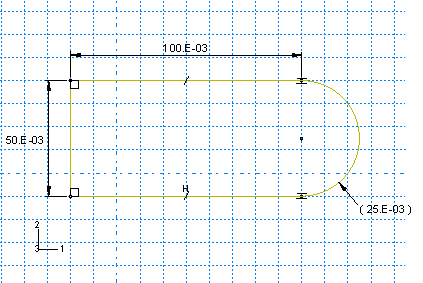
Sketches are two-dimensional profiles that form the geometry of features defining an Abaqus/CAE native part. You use the Sketcher to create these sketches, as shown in Figure 1–2. The Sketcher displays major gridlines in a solid line style and the X- and Y-axes of the sketch and minor gridlines in a dashed line style. In order to visually distinguish the part sketch from the Sketcher grid, the gridlines in most of the Sketcher figures in this guide are dashed.
View orientation triad
By default, Abaqus/CAE uses the alphabetical option, x-y-z, for labeling the view orientation triad. In general, this guide adopts the numerical option, 1-2-3, to permit direct correspondence with degree of freedom and output labeling. The view orientation triad is shown in the lower left corner of Figure 1–2.
Figure 1–3 shows the mouse button orientation for a left-handed and a right-handed 3-button mouse.
The following terms describe actions you perform using the mouse:Click
Press and quickly release the mouse button. Unless otherwise specified, the instruction "click" means that you should click mouse button 1.
Drag
Press and hold down mouse button 1 while moving the mouse.
Point
Move the mouse until the cursor is over the desired item.
Select
Point to an item and then click mouse button 1.
[Shift] + Click
Press and hold the [Shift] key, click mouse button 1, and then release the [Shift] key.
[Ctrl] + Click
Press and hold the [Ctrl] key, click mouse button 1, and then release the [Ctrl] key.
Abaqus/CAE is designed for use with a 3-button mouse. Accordingly, this guide refers to mouse buttons 1, 2, and 3 as shown in Figure 1–3. However, you can use Abaqus/CAE with a 2-button mouse as follows:
The two mouse buttons are equivalent to mouse buttons 1 and 3 on a 3-button mouse.
Pressing both mouse buttons simultaneously is equivalent to pressing mouse button 2 on a 3-button mouse.
Tip: You are instructed to click mouse button 2 in procedures throughout this guide. Make sure that you configure mouse button 2 (or the wheel button) to act as a middle button click.