To create a part:

1. In the Model Tree, under the model fluid-cfd, double-click Parts to create a new part. In the Create Part dialog box, name the part fluid, select Swept solid as the base feature, and 0.5 as the approximate size. Click Continue.

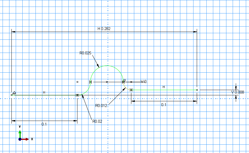
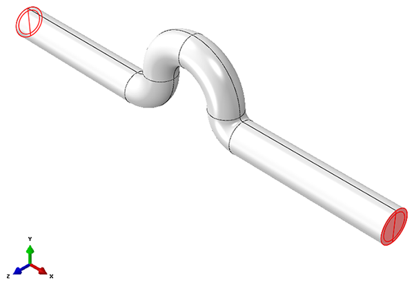
2. Sketch the sweep path for the part. Use the dimensions given in Figure E–2 to sketch a sweep path.

   Figure E–2 Sweep path for the fluid part.

   

3. Click Done in the prompt area.

4. Create a section sketch that will be swept along the sketched path to create a part. Enter 0.1 as the maximum scale for the section sketch.

5. Create the profile for the circular section as shown in Figure E–3. Place the center of the circle at the origin and the perimeter point along the Y- or Z-axis.

   Figure E–3 Section for the fluid part.

   

6. Click Done in the prompt area.

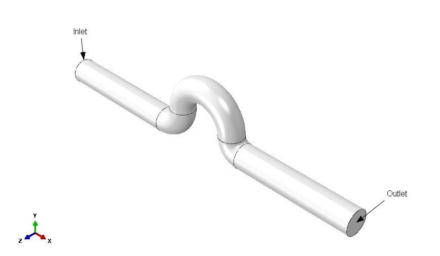
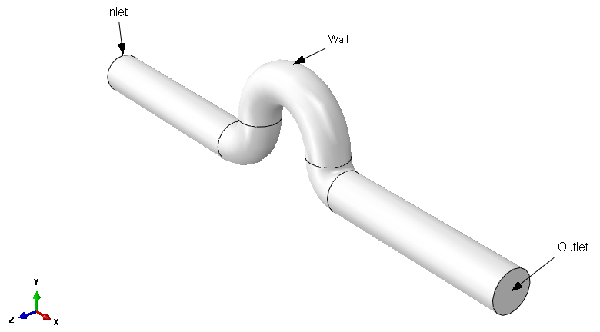
   Abaqus/CAE creates the part representing the fluid domain, as shown in Figure E–4. The inlet and outlet faces are indicated in the figure.

   Figure E–4 Fluid part.

   

To partition the part:

1. In the Model Tree, expand the fluid item under the Parts container, and double-click Mesh in the menu that appears to switch to the Mesh module.

   The part is initially colored orange, which means that it cannot be meshed using the default hexahedral element shape.

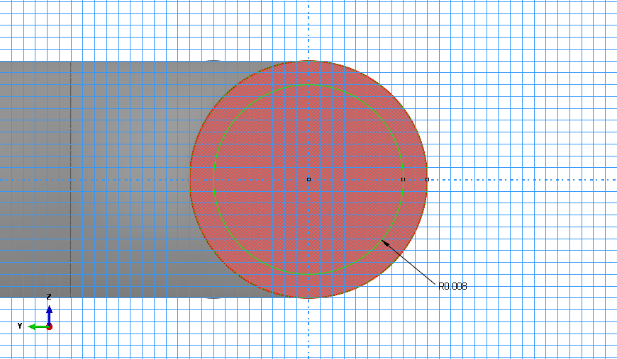
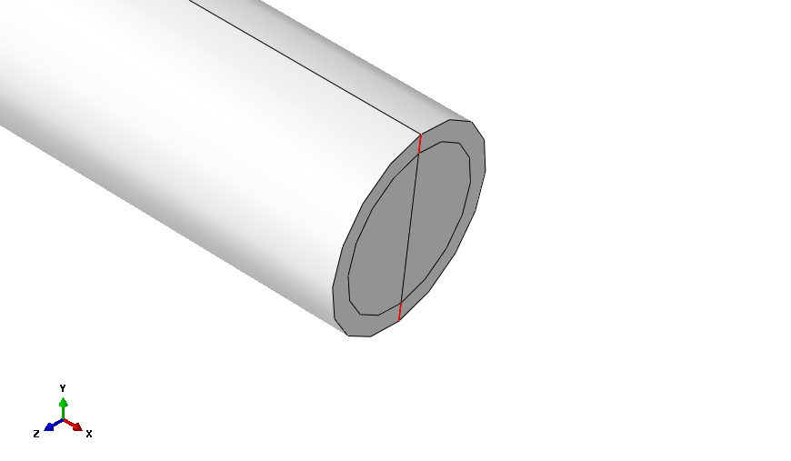
2. Use the Partition Face: Sketch tool to create a sketch of a circular section that will partition the inlet face. Place the center of the circle at the origin and the perimeter point along the Y- or Z-axis. The dimensions of the sketch are shown in Figure E–5.

   Figure E–5 Face partition sketch.

   

3. Create a partition cutting midway through the entire part in the X–Y plane, as shown in Figure E–6.

   Figure E–6 Partition along X–Y plane.

   

   1. Click the Partition Cell: Define Cutting Plane tool , and select Normal To Edge in the prompt area to specify the cutting plane.

   2. When prompted to select an edge, select the outer circular edge at the inlet.

   3. When prompted to select a point on the edge, select a point on the edge on the vertical Y-axis.

   4. Click Create Partition in the prompt area to complete the first partition.

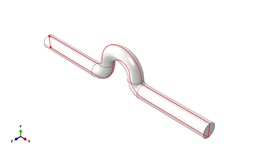
4. Use the circular partition on the inlet face to make a swept cut along the entire length of the tube, as shown in Figure E–7.

   Figure E–7 Partition of cylindrical core.

   

   1. Click and hold the Partition Cell tool to reveal additional tools, and select the Partition Cell: Extrude/Sweep Edges tool .

   2. Select the entire part, and click Done in the prompt area.

   3. In the prompt area, choose the by edge angle selection technique. Accept the default angle of 20.0.

   4. Select the circular edge created by the face partition on the inlet face, and click Done.

   5. Click Sweep Along Edge as the sweep method. Select the top edge of the straight section containing the inlet. This edge was created by the partition in the previous step.

   6. Click Create Partition.

      Abaqus/CAE adds a cylindrical core in the straight section of the tube. Repeat the process four more times to extend the cylindrical core throughout the entire length of the tube.

5. Create additional partitions along the length of the tube.

   1. Click the Partition Cell: Define Cutting Plane tool .

   2. Select the entire part, and click Done in the prompt area.

   3. Click Point & Normal in the prompt area to specify the cutting plane.

   4. When prompted to select a point, select the point on the outer circumferential edge between the straight section containing the outlet and its adjacent curved section, as shown in Figure E–8.

   5. Click Create Partition in the prompt area.

   6. When prompted to select an edge, select the straight edge indicated in Figure E–8.

      Figure E–8 Partition using straight edge to define normal.

      

   7. Repeat the procedure for the straight section attached to the inlet.

   8. For the curved section in the center of the part, use the 3 Points method to define a cutting plane, as indicated in Figure E–9.

      Figure E–9 Partition using 3 points method.

      

6. Partition the curved sections in the center of the part using the Normal to Edge method. Select the outer circular edge and the point midway along the edge to define the plane. The partition is shown in Figure E–10.

To define sets:

1. In the Model Tree, expand the container for the part named fluid and double-click Sets.

2. In the Create Set dialog box, name the set all and click Continue.

3. Select the entire geometry in the viewport, and click Done in the prompt area.

   Abaqus/CAE creates a set that contains the entire part.

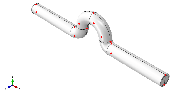
4. Repeat this procedure to create a set named fixed containing the faces at the inlet and outlet sections of the fluid domain, as shown in Figure E–10.

   Figure E–10 Set fixed.

   

5. Create a set named seed-1 containing the straight edges running radially through the tube between the central core and the outer surface, as indicated in Figure E–11 and Figure E–12. This set will be used to assign mesh seeds.

   Tip:  Switch to the wireframe view to facilitate your selections.

   Figure E–11 Set seed-1.

   

   Figure E–12 Close-up view of set seed-1.

   

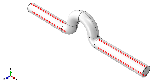
6. Create a set named seed-2 containing the straight edges running axially through the tube, as indicated in Figure E–13. This set will also be used to assign mesh seeds.

   Figure E–13 Set seed-2.

   

To define surfaces:

1. In the Model Tree, expand the container for the part named fluid and double-click Surfaces.

2. In the Create Surface dialog box, name the surface inlet and click Continue.

3. In the prompt area, select by angle as the selection technique. Select the faces at the inlet of the tube (Figure E–14 depicts the location of the surface).

4. Click Done in the prompt area.

5. Repeat the previous steps to create a surface named outlet at the outlet of the tube.

6. Repeat the previous steps to create a surface named wall representing the outer surface of the tube (excluding the inlet and outlet).

   Figure E–14 Surface definitions for the tube.

   

To define material properties:

1. In the Model Tree, double-click Materials to create a new material named fluid.

2. From the material editor, select GeneralDensity and specify a density value of 1000 kg/m³.

3. From the material editor, select MechanicalViscosity and specify a viscosity value of 0.001 Pa∙sec.

4. Click OK.

   Abaqus/CAE creates the material definition.

To define the CFD section:

1. In the Model Tree, double-click Sections to create a new section named fluid. Accept the default selection of a homogeneous fluid section, and click Continue.

2. In the Edit Section dialog box, select fluid as the material and click OK.

   Abaqus/CAE creates a fluid section definition.

To assign the CFD section:

1. In the Model Tree, expand the Parts container and the fluid container under it, then double-click Section Assignments.

2. In the prompt area, click Sets. In the Region Selection dialog box, choose all and click Continue.

3. Click OK in the section assignment editor.

To mesh the fluid domain:

1. In the Model Tree, expand the container for the part named fluid and double-click Mesh. Note that the core partition of the tube is colored yellow, while the outside cells are colored green; these color cues mean that the core can be meshed with a sweep meshing technique, while the outside cells can be meshed using a structured meshing technique.

2. Before meshing the part, assign mesh seeds. This seeding method creates a mesh that is finer near the walls of the tube and becomes coarser radially inward.

   First create seeds for the outside cells.

   1. Click the Seed Edges tool , and then click Sets/Surfaces in the prompt area (if necessary).

   2. In the Region Selection dialog box, select seed-1 as the set and click Continue.

   3. In the Local Seeds dialog box, select By size as the method, Single as the bias type, and enter 0.0004 as the minimum size and 0.001 as the maximum size.

   4. Zoom in to ensure that the seeds are concentrated near the wall. You can verify seed placement by confirming that the arrow indicating the bias direction points radially outward for each edge in the selected set.

   5. If any arrow points radially inward, you can flip it by clicking Select next to Flip bias and selecting the edges where the bias direction needs to be flipped.

3. Create seeds along the length of the tube.

   1. Follow the steps outlined above to create biased seeds that ensure coarser seeding at the inlet and outlet and finer seeds at the sections where the straight tube sections transition to the curved sections.

   2. In the Region Selection dialog box, select seed-2 as the set and click Continue.

   3. In the Local Seeds dialog box, select By size as the method, Single as the bias type, and enter 0.0035 as the minimum size and 0.01 as the maximum size.

   4. Ensure that each arrow points axially inward on both the inlet as well as the outlet sides of the tube. Flip the direction of any arrow that violates this condition.

4. Set the global seed size.

   1. Click the Seed Part tool . In the Global Seeds dialog box, enter 0.0025 as the approximate global size.

   2. Accept all other default values, and click OK.

      Abaqus/CAE sets the global seed size for the entire part.

5. Use the medial axis algorithm for the swept mesh regions of the part.

   1. Use the Display Group toolbar to display only the inner core of the tube (colored yellow).

      Tip:  Choose Cells as the selection method, and remove the outer regions of the part.

   2. Click the Mesh Controls tool, and assign the Medial axis mesh algorithm.

   3. Restore the visibility of all part regions.

6. Click the Mesh Part tool , and click Yes in the prompt area to create the part mesh.

   Abaqus/CAE displays the mesh, creating approximately 9000 elements.

To instance a part:

1. In the Model Tree, expand the Assembly container and double-click Instances in the list that appears to create an instance of the part.

2. In the Create Instance dialog box, select fluid from the Parts list and click OK.

To define an incompressible turbulent flow analysis step:

1. In the Model Tree, double-click Steps.

2. In the Create Step dialog box, accept Flow as the default procedure type and the default step name (Step–1). Click Continue.

3. From the Basic tabbed page of the step editor, do the following:

   1. Enter Flow in a rigid hose as the description.

   2. Enter 0.8 sec as the time period.

4. From the Incrementation tabbed page of the step editor, do the following:

   1. Accept Automatic (Fixed CFL) as the default time incrementation type.

   2. Enter 0.001 as the initial time increment.

   3. Enter 2.0 as the Maximum CFL number.

5. From the Solvers tabbed page of the step editor, accept the default settings on the Momentum Equation, Pressure Equation, and Transport Equation tabbed pages.

6. From the Turbulence tabbed page of the step editor, select Spalart-Allmaras as the turbulence model. Abaqus/CAE will use the Spalart-Allmaras turbulence model for turbulent flow calculations.

7. Click OK to close the Create Step dialog box.

To define output requests:

1. In the Model Tree, expand the Field Output Requests container. Note that a default field output request named F-Output-1 was created automatically at the time the step was created.

2. Double-click F-Output-1. Note that the output is requested at 20 evenly spaced time intervals.

3. Delete the preselected output, and select the following output variables: V, PRESSURE, DIV, TURBNU, and VORTICITY.

4. Click OK to close the output request editor.

To define boundary conditions:

1. Define an inlet boundary condition at the inlet surface.

   1. In the Model Tree, double-click BCs.

   2. Name the boundary condition inlet, and select Step-1 as the step.

   3. Select Fluid as the category and Fluid inlet/outlet as the type.

   4. Select fluid-1.inlet as the surface to which the boundary condition will be applied (click Surfaces in the prompt area if necessary).

   5. From the Momentum tabbed page of the boundary condition editor, toggle on Specify and select Velocity.

   6. Set the X-velocity component V1 to 1. Set the Y- and Z-velocity components V2 and V3 to 0.

   7. From the Turbulence tabbed page, toggle on Kinematic eddy viscosity and enter a value of 5e–6. Abaqus/CAE sets the inlet turbulence of the flow.

   8. Click OK to create the boundary condition and to close the boundary condition editor.

2. Define an outlet boundary condition at the outlet surface.

   1. In the Model Tree, double-click BCs.

   2. Name the boundary condition outlet, and select Step-1 as the step.

   3. Select Fluid as the category and Fluid inlet/outlet as the type.

   4. Select fluid-1.outlet as the surface to which the boundary condition will be applied.

   5. From the Momentum tabbed page of the boundary condition editor, toggle on Specify and select Pressure.

   6. Set the pressure to 0.

   7. Click OK to create the boundary condition and to close the boundary condition editor.

3. Define a no-slip/no-penetration boundary condition at the cylinder surface.

   1. In the Model Tree, double-click BCs.

   2. Name the boundary condition noSlip, and select Step-1 as the step.

   3. Select Fluid as the category and Fluid wall condition as the type.

   4. Select fluid-1.wall as the surface to which the boundary condition will be applied.

   5. Select No slip as the condition.

   6. Click OK to close the boundary condition editor.

      Abaqus/CAE creates the no-slip/no-penetration boundary condition.

To specify a predefined field for the turbulent viscosity:

1. In the Model Tree, double-click Predefined Fields.

2. Name the initial condition initial turbulence, and select Initial as the step.

3. Select Fluid as the category and Fluid turbulence as the type.

4. Set the Kinematic eddy viscosity to 5e–6.

5. Click OK to close the predefined field editor.

   Abaqus/CAE creates the predefined field for turbulent viscosity.

To request surface output quantities:

1. In the Model Tree, click mouse button 3 on the fluid-cfd model and select Edit Keywords from the menu that appears.

   The keywords editor appears.

2. Scroll down, and click in the *Output, field option block.

3. Click Add After, and enter the following:

   *Surface output, surface=fluid-1.wall
    yplus

4. Navigate to the *Output, history option block, and change the output frequency to 1.

5. Click Add after, and enter the following:

   *Surface output, surface=fluid-1.inlet
    massflow,
   *Surface output, surface=fluid-1.outlet
    massflow,

6. Click OK to close the keywords editor.

   Abaqus/CAE modifies the selected output requests.