Products: Abaqus/Standard Abaqus/Explicit
The parallel rheological framework:
is intended for modeling polymers and elastomeric materials that exhibit permanent set and nonlinear viscous behavior and undergo large deformations;
consists of multiple viscoelastic networks and, optionally, an elastoplastic network in parallel;
uses a hyperelastic material model to specify the elastic response;
can be combined with Mullins effect;
bases the elastoplastic response on multiplicative split of the deformation gradient and the theory of incompressible isotropic hardening plasticity;
can include nonlinear kinematic hardening with multiple backstresses in the elastoplastic response in Abaqus/Standard; and
uses multiplicative split of the deformation gradient and a flow rule derived from a creep potential to specify the viscous behavior.
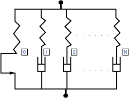
The parallel rheological framework allows definition of a nonlinear viscoelastic-elastoplastic model consisting of multiple networks connected in parallel, as shown in Figure 22.8.2–1.
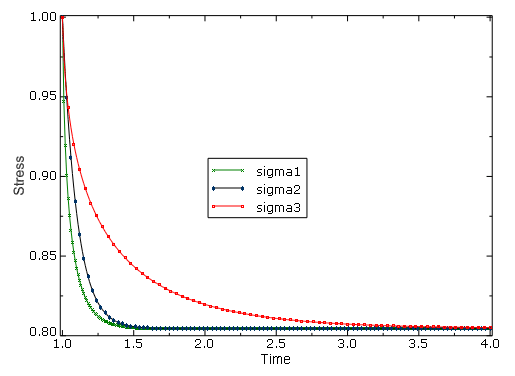
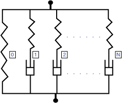
The number of viscoelastic networks, N, can be arbitrary; however, at most one equilibrium network (networkThe model can be used to predict complex behavior of materials subjected to finite strains, which cannot be modeled accurately using other models available in Abaqus. An example of such complex behavior is depicted in Figure 22.8.2–2, which shows normalized stress relaxation curves for three different strain levels. This behavior can be modeled accurately using the nonlinear viscoelastic model depicted in Figure 22.8.2–3, which can be defined within the framework; but it cannot be captured with the linear viscoelastic model (see “Time domain viscoelasticity,” Section 22.7.1). In the latter case, the three curves would coincide.
The elastic part of the response for all the networks is specified using the hyperelastic material model. Any of the hyperelastic models available in Abaqus can be used (see “Hyperelastic behavior of rubberlike materials,” Section 22.5.1). The same hyperelastic material definition is used for all the networks, scaled by a stiffness ratio specific to each network. Consequently, only one hyperelastic material definition is required by the model along with the stiffness ratio for each network. The elastic response can be specified by defining either the instantaneous response or the long-term response.
In addition to the elastic response described above, the response of the equilibrium network can include plasticity and Mullins effect to predict material softening. If the plastic response is defined using isotropic hardening, the response in the equilibrium network is equivalent to that of the permanent set model available in Abaqus (see “Permanent set in rubberlike materials,” Section 23.7.1, for a detailed description of the model). In Abaqus/Standard the nonlinear kinematic hardening model with multiple backstresses can be specified in addition to isotropic plastic hardening. The nonlinear kinematic hardening model is a generalization of the model used for metal plasticity. See “Models for metals subjected to cyclic loading,” Section 23.2.2, for a detailed description of the model, with the difference that the Cauchy stress is replaced with the Kirchhoff stress in the current formulation.
Viscous behavior must be defined for each viscoelastic network. It is modeled by assuming the multiplicative split of the deformation gradient and the existence of the creep potential, ![]() , from which the flow rule is derived. In the multiplicative split the deformation gradient is expressed as
, from which the flow rule is derived. In the multiplicative split the deformation gradient is expressed as
![]()
![]()
![]()
![]()
![]()
![]()
The power law model is available in the form
![]()
is the equivalent creep strain rate,
![]()
is the equivalent creep strain,
![]()
is the equivalent deviatoric Kirchhoff stress,
![]()
is the Kirchhoff pressure, and
![]() , m, n, a and
, m, n, a and ![]()
are material parameters.
The power-law strain hardening model is available in the form
![]()
is the equivalent creep strain rate,
![]()
is the equivalent creep strain,
![]()
is the equivalent deviatoric Kirchhoff stress, and
A, m, and n
are material parameters.
The hyperbolic-sine law is available in the form
![]()
![]() and
and ![]()
are defined above, and
A, B, and n
are material parameters.
The Bergstrom-Boyce model is available in the form
![]()
![]()
![]() and
and ![]()
are defined above, and
A, m, C, and E
are material parameters.
The response of the network defined by the Bergstrom-Boyce model is very similar to the response of the time-dependent network in the hysteresis model (see “Hysteresis in elastomers,” Section 22.8.1). However, there are also important differences between the models. In the Bergstrom-Boyce model the equivalent Kirchhoff stress is used instead of the equivalent Cauchy stress, which is used in the hysteresis model. (The two stress measures become equivalent for the case of incompressible materials.) In addition, the material parameters, A, in the models differ by a factor of ![]() . The parameter in the hysteresis model must be multiplied by
. The parameter in the hysteresis model must be multiplied by ![]() to make the parameters equivalent.
to make the parameters equivalent.
A user-defined creep model is available of the following general form:
![]()
![]()
![]()
is the first invariant of ![]() ,
,
![]()
is the second invariant of ![]() ,
,
![]() ,
, ![]() ,
, ![]() ,
, ![]() and
and ![]()
are defined above,
t
is the time,
![]()
is the temperature, and
FV
are field variables.
Only isotropic thermal expansion is permitted with nonlinear viscoelastic materials (“Thermal expansion,” Section 26.1.2).
The nonlinear viscoelastic response is defined by specifying the identifier, stiffness ratio, and creep law for each viscoelastic network.
Each viscoelastic network in the material model must be assigned a unique network identifier or network id. The network identifiers must be consecutive integers starting with 1. The order in which they are specified is not important.
| Input File Usage: | Use the following option to specify the network identifier: |
*VISCOELASTIC, NONLINEAR, NETWORKID=networkId |
The contribution of each network to the overall response of the material is determined by the value of the stiffness ratio, ![]() , which is used to scale the elastic response of the network material. The sum of the stiffness ratios of the viscoelastic networks must be smaller than or equal to 1. If the sum of the ratios is equal to 1, the purely elastic equilibrium network is not created. If the sum of the ratios is smaller than 1, the equilibrium network is created with a stiffness ratio,
, which is used to scale the elastic response of the network material. The sum of the stiffness ratios of the viscoelastic networks must be smaller than or equal to 1. If the sum of the ratios is equal to 1, the purely elastic equilibrium network is not created. If the sum of the ratios is smaller than 1, the equilibrium network is created with a stiffness ratio, ![]() , equal to
, equal to
You can specify that the stiffness ratio remains constant during the analysis:
| Input File Usage: | *VISCOELASTIC, NONLINEAR, SRATIO=ratio |
Alternatively, you can define the stiffness ratio as a function of temperature and predefined field variables.
| Input File Usage: | *NETWORK STIFFNESS RATIO, N=nNetworks, DEPENDENCIES=n |
The definition of creep behavior in Abaqus/Standard is completed by specifying the creep law.
The power law model is defined by specifying five material parameters: ![]() , n, m, a, and
, n, m, a, and ![]() . The parameter
. The parameter ![]() must be positive. It is introduced for dimensional consistency, and its default value is 1.0. For physically reasonable behavior
must be positive. It is introduced for dimensional consistency, and its default value is 1.0. For physically reasonable behavior ![]() and n must be positive, a must be nonnegative (the default is 0.0), and 1 < m ≤ 0.
and n must be positive, a must be nonnegative (the default is 0.0), and 1 < m ≤ 0.
| Input File Usage: | *VISCOELASTIC, NONLINEAR, LAW=POWER LAW |
The strain hardening law is defined by specifying three material parameters: A, n, and m. For physically reasonable behavior A and n must be positive and 1 < m ≤ 0.
| Input File Usage: | *VISCOELASTIC, NONLINEAR, LAW=STRAIN |
The hyperbolic sine creep law is specified by providing three nonnegative parameters: A, B, and n.
| Input File Usage: | *VISCOELASTIC, NONLINEAR, LAW=HYPERB |
The Bergstrom-Boyce creep law is specified by providing four parameters: A, m, C, and E. The parameters A and E must be nonnegative, the parameter m must be positive, and the parameter C must lie in ![]() .
.
| Input File Usage: | *VISCOELASTIC, NONLINEAR, LAW=BERGSTROM-BOYCE |
An alternative method for defining the creep law involves using user subroutine UCREEPNETWORK in Abaqus/Standard or VUCREEPNETWORK in Abaqus/Explicit. Optionally, you can specify the number of property values needed as data in the user subroutine.
| Input File Usage: | *VISCOELASTIC, NONLINEAR, LAW=USER, PROPERTIES=n |
Depending on the choice of units, the value of A in the strain power-law, hyperbolic-sine, and Bergstrom-Boyce models may be very small for typical creep strain rates. If A is less than 1027, numerical difficulties can cause errors in the material calculations; therefore, a different system of units should be used to avoid such difficulties in the calculation of creep strain increments. In such cases it is recommended to replace the strain power-law model with the power law model, which does not have the limitation described above. The strain power-law model is a special case of the power law model obtained by setting ![]() ,
, ![]() , and
, and ![]() .
.
Thermo-rheologically simple temperature effects can be included for each viscoelastic network. In this case the creep law is modified and takes the following form:
![]()
![]()
An alternative method for specifying the shift function involves using user subroutine UTRSNETWORK. Optionally, you can specify the number of property values needed as data in the user subroutine.
| Input File Usage: | *TRS, DEFINITION=USER, PROPERTIES=n |
In Abaqus/Standard the material is active during all stress/displacement procedure types. However, the creep effects are taken into account only in quasi-static (“Quasi-static analysis,” Section 6.2.5), coupled temperature-displacement (“Fully coupled thermal-stress analysis,” Section 6.5.3), direct-integration implicit dynamic (“Implicit dynamic analysis using direct integration,” Section 6.3.2), and steady-state transport (“Steady-state transport analysis,” Section 6.4.1) analyses. If the material is used in a steady-state transport analysis, it cannot include plasticity. In other stress/displacement procedures the evolution of the state variables is suppressed and the creep strain remains unchanged. In Abaqus/Explicit the creep effects are always active.
The nonlinear viscoelastic model is available with continuum elements that include mechanical behavior (elements that have displacement degrees of freedom), except for one-dimensional and plane stress elements.
In addition to the standard output identifiers available in Abaqus (“Abaqus/Standard output variable identifiers,” Section 4.2.1, and “Abaqus/Explicit output variable identifiers,” Section 4.2.2), the following variables have special meaning for the nonlinear viscoelastic material model:
CEEQ | The overall equivalent creep strain, defined as |
CE | The overall creep strain, defined as |
CENER | The overall viscous dissipated energy per unit volume, defined as |
SENER | The overall elastic strain energy density per unit volume, defined as |
SNETk | All stress components in the |
If plasticity is specified in the equilibrium network, the standard output identifiers available in Abaqus corresponding to other isotropic and kinematic hardening plasticity models can be obtained for this model as well. In addition, if the Mullins effect is used in the model, the output variables available for the Mullins effect model (see “Mullins effect,” Section 22.6.1) can be requested.
Bergstrom, J. S., and M. C. Boyce, “Constitutive Modeling of the Large Strain Time-Dependent Behavior of Elastomers,” Journal of the Mechanics and Physics of Solids, vol. 46, pp. 931–954, 1998.
Bergstrom, J. S., and M. C. Boyce, “Large Strain Time-Dependent Behavior of Filled Elastomers,” Mechanics of Materials, vol. 32, pp. 627–644, 2000.
Bergstrom, J. S., and J. E. Bischoff, “An Advanced Thermomechanical Constitutive Model for UHMWPE,” International Journal of Structural Changes in Solids, vol. 2, pp. 31–39, 2010.
Hurtado, J. A., I. Lapczyk, and S. M. Govindarajan, “Parallel Rheological Framework to Model Non-Linear Viscoelasticity, Permanent Set, and Mullins Effect in Elastomers,” Constitutive Models for Rubber VIII 95, 2013.
Lapczyk, I., J. A. Hurtado, and S. M. Govindarajan, “A Parallel Rheological Framework for Modeling Elastomers and Polymers,” 182nd Technical Meeting of the Rubber Division of the American Chemical Society, pp. 1840–1859, October 2012, Cincinnati, OH.