Products: Abaqus/Standard Abaqus/CAE Abaqus/Viewer
Modeling discontinuities, such as cracks, as an enriched feature:
is commonly referred to as the extended finite element method (XFEM);
is an extension of the conventional finite element method based on the concept of partition of unity;
allows the presence of discontinuities in an element by enriching degrees of freedom with special displacement functions;
enables the modeling of discontinuities in the fluid pressure field as well as fluid flow within the cracked element surfaces as in hydraulically driven fracture;
does not require the mesh to match the geometry of the discontinuities;
is a very attractive and effective way to simulate initiation and propagation of a discrete crack along an arbitrary, solution-dependent path without the requirement of remeshing in the bulk materials;
can be simultaneously used with the surface-based cohesive behavior approach (see “Surface-based cohesive behavior,” Section 37.1.10) or the Virtual Crack Closure Technique (see “Crack propagation analysis,” Section 11.4.3), which are best suited for modeling interfacial delamination;
can be performed using the static procedure (see “Static stress analysis,” Section 6.2.2), the implicit dynamic procedure (see “Implicit dynamic analysis using direct integration,” Section 6.3.2), the low-cycle fatigue analysis using the direct cyclic approach (see “Low-cycle fatigue analysis using the direct cyclic approach,” Section 6.2.7), the geostatic stress field procedure (see “Geostatic stress state,” Section 6.8.2), or coupled pore fluid diffusion/stress analysis (see “Coupled pore fluid diffusion and stress analysis,” Section 6.8.1);
can also be used to perform contour integral evaluations for an arbitrary stationary surface crack without the need to refine the mesh around the crack tip;
allows contact interaction of cracked element surfaces based on a small-sliding formulation;
allows the application of distributed pressure loads to the cracked element surfaces;
allows the output of some surface variables on the cracked element surfaces;
allows both material and geometrical nonlinearity; and
is available only for first-order stress/displacement solid continuum elements, first-order displacement/pore pressure solid continuum elements, and second-order stress/displacement tetrahedron elements.
Modeling stationary discontinuities, such as a crack, with the conventional finite element method requires that the mesh conforms to the geometric discontinuities. Therefore, considerable mesh refinement is needed in the neighborhood of the crack tip to capture the singular asymptotic fields adequately. Modeling a growing crack is even more cumbersome because the mesh must be updated continuously to match the geometry of the discontinuity as the crack progresses.
The extended finite element method (XFEM) alleviates the shortcomings associated with meshing crack surfaces. The extended finite element method was first introduced by Belytschko and Black (1999). It is an extension of the conventional finite element method based on the concept of partition of unity by Melenk and Babuska (1996), which allows local enrichment functions to be easily incorporated into a finite element approximation. The presence of discontinuities is ensured by the special enriched functions in conjunction with additional degrees of freedom. However, the finite element framework and its properties such as sparsity and symmetry are retained.
For the purpose of fracture analysis, the enrichment functions typically consist of the near-tip asymptotic functions that capture the singularity around the crack tip and a discontinuous function that represents the jump in displacement across the crack surfaces. The approximation for a displacement vector function ![]() with the partition of unity enrichment is
with the partition of unity enrichment is
Figure 10.7.1–1 illustrates the asymptotic crack tip functions in an isotropic elastic material, ![]() , which are given by
, which are given by
![]()
These functions span the asymptotic crack-tip function of elasto-statics, and ![]() takes into account the discontinuity across the crack face. The use of asymptotic crack-tip functions is not restricted to crack modeling in an isotropic elastic material. The same approach can be used to represent a crack along a bimaterial interface, impinged on the bimaterial interface, or in an elastic-plastic power law hardening material. However, in each of these three cases different forms of asymptotic crack-tip functions are required depending on the crack location and the extent of the inelastic material deformation. The different forms for the asymptotic crack-tip functions are discussed by Sukumar (2004), Sukumar and Prevost (2003), and Elguedj (2006), respectively.
takes into account the discontinuity across the crack face. The use of asymptotic crack-tip functions is not restricted to crack modeling in an isotropic elastic material. The same approach can be used to represent a crack along a bimaterial interface, impinged on the bimaterial interface, or in an elastic-plastic power law hardening material. However, in each of these three cases different forms of asymptotic crack-tip functions are required depending on the crack location and the extent of the inelastic material deformation. The different forms for the asymptotic crack-tip functions are discussed by Sukumar (2004), Sukumar and Prevost (2003), and Elguedj (2006), respectively.
Accurately modeling the crack-tip singularity requires constantly keeping track of where the crack propagates and is cumbersome because the degree of crack singularity depends on the location of the crack in a non-isotropic material. Therefore, we consider the asymptotic singularity functions only when modeling stationary cracks in Abaqus/Standard. Moving cracks are modeled using one of the two alternative approaches described below.
One alternative approach within the framework of XFEM is based on traction-separation cohesive behavior. This approach is used in Abaqus/Standard to simulate crack initiation and propagation. This is a very general interaction modeling capability, which can be used for modeling brittle or ductile fracture. The other crack initiation and propagation capabilities available in Abaqus/Standard are based on cohesive elements (“Defining the constitutive response of cohesive elements using a traction-separation description,” Section 32.5.6) or on surface-based cohesive behavior (“Surface-based cohesive behavior,” Section 37.1.10). Unlike these methods, which require that the cohesive surfaces align with element boundaries and the cracks propagate along a set of predefined paths, the XFEM-based cohesive segments method can be used to simulate crack initiation and propagation along an arbitrary, solution-dependent path in the bulk materials, since the crack propagation is not tied to the element boundaries in a mesh. In this case the near-tip asymptotic singularity is not needed, and only the displacement jump across a cracked element is considered. Therefore, the crack has to propagate across an entire element at a time to avoid the need to model the stress singularity.
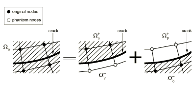
Phantom nodes, which are superposed on the original real nodes, are introduced to represent the discontinuity of the cracked elements, as illustrated in Figure 10.7.1–2. When the element is intact, each phantom node is completely constrained to its corresponding real node. When the element is cut through by a crack, the cracked element splits into two parts. Each part is formed by a combination of some real and phantom nodes depending on the orientation of the crack. Each phantom node and its corresponding real node are no longer tied together and can move apart.
The magnitude of the separation is governed by the cohesive law until the cohesive strength of the cracked element is zero, after which the phantom and the real nodes move independently. To have a set of full interpolation bases, the part of the cracked element that belongs in the real domain, ![]() , is extended to the phantom domain,
, is extended to the phantom domain, ![]() . Then the displacement in the real domain,
. Then the displacement in the real domain, ![]() , can be interpolated by using the degrees of freedom for the nodes in the phantom domain,
, can be interpolated by using the degrees of freedom for the nodes in the phantom domain, ![]() . The jump in the displacement field is realized by simply integrating only over the area from the side of the real nodes up to the crack; i.e.,
. The jump in the displacement field is realized by simply integrating only over the area from the side of the real nodes up to the crack; i.e., ![]() and
and ![]() . This method provides an effective and attractive engineering approach and has been used for simulation of the initiation and growth of multiple cracks in solids by Song (2006) and Remmers (2008). It has been proven to exhibit almost no mesh dependence if the mesh is sufficiently refined.
. This method provides an effective and attractive engineering approach and has been used for simulation of the initiation and growth of multiple cracks in solids by Song (2006) and Remmers (2008). It has been proven to exhibit almost no mesh dependence if the mesh is sufficiently refined.
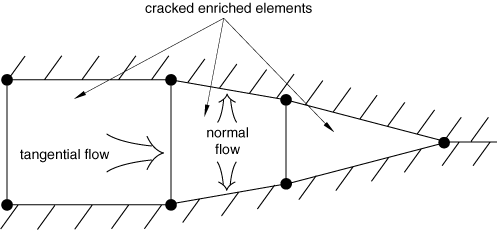
The cohesive segments method in conjunction with phantom nodes discussed above can also be extended to model hydraulically driven fracture. In this case additional phantom nodes with pore pressure degrees of freedom are introduced on the edges of each enriched element to model the fluid flow within the cracked element surfaces in conjunction with the phantom nodes that are superposed on the original real nodes to represent the discontinuities of displacement and fluid pressure in a cracked element. The phantom node at each element edge is not activated until the edge is intersected by a crack. The flow patterns of the pore fluid in the cracked elements are shown in Figure 10.7.1–3. The fluid is assumed to be incompressible. The fluid flow continuity, which accounts for both tangential and normal flow within and across the cracked element surfaces as well as the rate of opening of the cracked element surfaces, is maintained. The fluid pressure on the cracked element surfaces contributes to the traction-separation behavior of the cohesive segments in the enriched elements, which enables the modeling of hydraulically driven fracture.
Another alternative approach to modeling moving cracks within the framework of XFEM is based on the principles of linear elastic fracture mechanics (LEFM). Therefore, it is more appropriate for problems in which brittle crack propagation occurs. Similar to the XFEM-based cohesive segments method described above, the near-tip asymptotic singularity is not considered, and only the displacement jump across a cracked element is considered. Therefore, the crack has to propagate across an entire element at a time to avoid the need to model the stress singularity. The strain energy release rate at the crack tip is calculated based on the modified Virtual Crack Closure Technique (VCCT), which has been used to model delamination along a known and partially bonded surface (see “Crack propagation analysis,” Section 11.4.3). However, unlike this method, the XFEM-based LEFM approach can be used to simulate crack propagation along an arbitrary, solution-dependent path in the bulk material without the requirement of a pre-existing crack in the model.
The modeling technique is very similar to the XFEM-based cohesive segment approach described above where phantom nodes are introduced to represent the discontinuity of the cracked element when the fracture criterion is satisfied. The real node and the corresponding phantom node will separate when the equivalent strain energy release rate exceeds the critical strain energy release rate at the crack tip in an enriched element. The traction is initially carried as equal and opposite forces on the two surfaces of the cracked element. The traction is ramped down linearly over the separation between the two surfaces with the dissipated strain energy equal to either the critical strain energy required to initiate the separation or the critical strain energy required to propagate the crack depending on whether the VCCT or the enhanced VCCT criterion is specified.
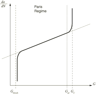
The XFEM-based LEFM approach can also be used to simulate a discrete crack growth subjected to sub-critical cyclic loading in a low-cycle fatigue analysis using the direct cyclic approach (“Low-cycle fatigue analysis using the direct cyclic approach,” Section 6.2.7). The fracture energy release rates at the crack tips in the enriched elements are calculated based on the above mentioned modified VCCT technique. The onset and crack growth are characterized by using the Paris law, which relates the relative fracture energy release rates to crack growth rates as illustrated in Figure 10.7.1–4. This approach has been used to model progressive delamination under a sub-critical cyclic loading along a known and partially bonded surface (see “Low-cycle fatigue criterion” in “Crack propagation analysis,” Section 11.4.3). However, unlike this method, the XFEM-based LEFM approach can be used to simulate fatigue crack propagation along an arbitrary, solution-dependent path in the bulk material.
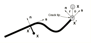
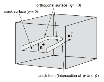
A key development that facilitates treatment of cracks in an extended finite element analysis is the description of crack geometry, because the mesh is not required to conform to the crack geometry. The level set method, which is a powerful numerical technique for analyzing and computing interface motion, fits naturally with the extended finite element method and makes it possible to model arbitrary crack growth without remeshing. The crack geometry is defined by two almost-orthogonal signed distance functions, as illustrated in Figure 10.7.1–5. The first, ![]() , describes the crack surface, while the second,
, describes the crack surface, while the second, ![]() , is used to construct an orthogonal surface so that the intersection of the two surfaces gives the crack front.
, is used to construct an orthogonal surface so that the intersection of the two surfaces gives the crack front. ![]() indicates the positive normal to the crack surface;
indicates the positive normal to the crack surface; ![]() indicates the positive normal to the crack front. No explicit representation of the boundaries or interfaces is needed because they are entirely described by the nodal data. Two signed distance functions per node are generally required to describe a crack geometry.
indicates the positive normal to the crack front. No explicit representation of the boundaries or interfaces is needed because they are entirely described by the nodal data. Two signed distance functions per node are generally required to describe a crack geometry.
You must specify an enriched feature and its properties. One or multiple pre-existing cracks can be associated with an enriched feature. In addition, during an analysis one or multiple cracks can initiate in an enriched feature without any initial defects. However, multiple cracks can nucleate in a single enriched feature only when the damage initiation criterion is satisfied in multiple elements in the same time increment. Otherwise, additional cracks will not nucleate until all the pre-existing cracks in an enriched feature have propagated through the boundary of the given enriched feature. If several crack nucleations are expected to occur at different locations sequentially during an analysis, multiple enriched features can be specified in the model. Enriched degrees of freedom are activated only when an element is intersected by a crack. Only stress/displacement or displacement/pore pressure solid continuum elements can be associated with an enriched feature.
| Input File Usage: | *ENRICHMENT |
| Abaqus/CAE Usage: | Interaction module: Special |
You can choose to model an arbitrary stationary crack or a discrete crack propagation along an arbitrary, solution-dependent path. The former requires that the elements around the crack tips are enriched with asymptotic functions to catch the singularity and that the elements intersected by the crack interior are enriched with the jump function across the crack surfaces. The latter infers that crack propagation is modeled with either the cohesive segments method or the linear elastic fracture mechanics approach in conjunction with phantom nodes. However, the options are mutually exclusive and cannot be specified simultaneously in a model.
| Input File Usage: | Use the following option to specify a crack propagation analysis (default): |
*ENRICHMENT, TYPE=PROPAGATION CRACK Use the following option to specify an analysis with stationary cracks: *ENRICHMENT, TYPE=STATIONARY CRACK |
| Abaqus/CAE Usage: | Use the following input to specify a crack propagation analysis: |
Interaction module: crack editor: toggle on Allow crack growth Use the following input to specify an analysis with stationary cracks: Interaction module: crack editor: toggle off Allow crack growth |
You must assign a name to an enriched feature, such as a crack. This name can be used in defining the initial location of the crack surfaces, in identifying a crack for contour integral output, in activating or deactivating the crack propagation analysis, and in generating cracked element surfaces.
| Input File Usage: | *ENRICHMENT, NAME=name |
| Abaqus/CAE Usage: | Interaction module: Special |
You must associate the enrichment definition with a region of your model. Only degrees of freedom in elements within these regions are potentially enriched with special functions. The region should consist of elements that are presently intersected by cracks and those that are likely to be intersected by cracks as the cracks propagate.
| Input File Usage: | *ENRICHMENT, ELSET=element set name |
| Abaqus/CAE Usage: | Interaction module: Special |
As a crack propagates through the model, a crack surface representing both facets of cracked elements is generated on those enriched elements that are intersected by a crack during the analysis. You must associate the name of an enriched feature with the surface (see “Assigning a name to the enriched feature,” above).
The generated crack surface is supported only for the application of distributed pressure loads and the output of some surface variables.
| Input File Usage: | *SURFACE, TYPE=XFEM |
| Abaqus/CAE Usage: | An XFEM-based crack surface is not supported in Abaqus/CAE. |
When an element is cut by a crack, the compressive behavior of the crack surfaces has to be considered. The formulae that govern behavior are very similar to those used for surface-based small-sliding penalty contact (“Mechanical contact properties: overview,” Section 37.1.1).
For an element intersected by a stationary crack or a moving crack with the linear elastic fracture mechanics approach, it is assumed that the elastic cohesive strength of the cracked element is zero. Therefore, compressive behavior of the crack surfaces is fully defined with the above options when the crack surfaces come into contact. For a moving crack with the cohesive segments method, the situation is more complex; traction-separation cohesive behavior as well as compressive behavior of the crack surfaces are involved in a cracked element. In the contact normal direction, the pressure-overclosure relationship governing the compressive behavior between the surfaces does not interact with the cohesive behavior, since they each describe the interaction between the surfaces in a different contact regime. The pressure-overclosure relationship governs the behavior only when the crack is “closed”; the cohesive behavior contributes to the contact normal stress only when the crack is “open” (i.e., not in contact).
If the elastic cohesive stiffness of an element is undamaged in the shear direction, it is assumed that the cohesive behavior is active. Any tangential slip is assumed to be purely elastic in nature and is resisted by the elastic cohesive strength of the element, resulting in shear forces. If damage has been defined, the cohesive contribution to the shear stresses starts degrading with damage evolution. Once maximum degradation has been reached, the cohesive contribution to the shear stresses is zero. The friction model activates and begins contributing to the shear stresses.
| Input File Usage: | Use the following options to define contact of crack surfaces using a small-sliding formulation: |
*ENRICHMENT, INTERACTION=interaction_property_name *SURFACE INTERACTION, NAME=interaction_property_name *SURFACE BEHAVIOR |
| Abaqus/CAE Usage: | Interaction module: crack editor: toggle on Specify contact property |
The formulae and laws that govern the behavior of XFEM-based cohesive segments for a crack propagation analysis are very similar to those used for cohesive elements with traction-separation constitutive behavior (“Defining the constitutive response of cohesive elements using a traction-separation description,” Section 32.5.6) and those used for surface-based cohesive behavior (“Surface-based cohesive behavior,” Section 37.1.10). The similarities extend to the linear elastic traction-separation model, damage initiation criteria, and damage evolution laws.
The available traction-separation model in Abaqus assumes initially linear elastic behavior followed by the initiation and evolution of damage. The elastic behavior is written in terms of an elastic constitutive matrix that relates the normal and shear stresses to the normal and shear separations of a cracked element.
The nominal traction stress vector, ![]() , consists of the following components:
, consists of the following components: ![]() ,
, ![]() , and (in three-dimensional problems)
, and (in three-dimensional problems) ![]() , which represent the normal and the two shear tractions, respectively. The corresponding separations are denoted by
, which represent the normal and the two shear tractions, respectively. The corresponding separations are denoted by ![]() ,
, ![]() , and
, and ![]() . The elastic behavior can then be written as
. The elastic behavior can then be written as
The normal and tangential stiffness components will not be coupled: pure normal separation by itself does not give rise to cohesive forces in the shear directions, and pure shear slip with zero normal separation does not give rise to any cohesive forces in the normal direction.
The terms ![]() ,
, ![]() , and
, and ![]() are calculated based on the elastic properties for an enriched element. Specifying the elastic properties of the material in an enriched region is sufficient to define both the elastic stiffness and the traction-separation behavior.
are calculated based on the elastic properties for an enriched element. Specifying the elastic properties of the material in an enriched region is sufficient to define both the elastic stiffness and the traction-separation behavior.
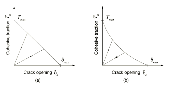
Damage modeling allows you to simulate the degradation and eventual failure of an enriched element. The failure mechanism consists of two ingredients: a damage initiation criterion and a damage evolution law. The initial response is assumed to be linear as discussed in the previous section. However, once a damage initiation criterion is met, damage can occur according to a user-defined damage evolution law. Figure 10.7.1–6 shows a typical linear and a typical nonlinear traction-separation response with a failure mechanism. The enriched elements do not undergo damage under pure compression.
Damage of the traction-separation response for cohesive behavior in an enriched element is defined within the same general framework used for conventional materials (see “Progressive damage and failure,” Section 24.1.1). However, unlike cohesive elements with traction-separation behavior, you do not have to specify the undamaged traction-separation behavior in an enriched element.
Crack initiation refers to the beginning of degradation of the cohesive response at an enriched element. The process of degradation begins when the stresses or the strains satisfy specified crack initiation criteria. Crack initiation criteria are available based on the following Abaqus/Standard built-in models:
the maximum principal stress criterion,
the maximum principal strain criterion,
the maximum nominal stress criterion,
the maximum nominal strain criterion,
the quadratic traction-interaction criterion, and
the quadratic separation-interaction criterion.
An additional crack is introduced or the crack length of an existing crack is extended after an equilibrium increment when the fracture criterion, f, reaches the value 1.0 within a given tolerance:
![]()
| Input File Usage: | *DAMAGE INITIATION, TOLERANCE= |
| Abaqus/CAE Usage: | Property module: material editor: Mechanical: Damage for Traction Separation Laws: Quade Damage, Maxe Damage, Quads Damage, Maxs Damage, Maxpe Damage, or Maxps Damage: Tolerance: |
When the maximum principal stress or the maximum principal strain criterion is specified, the newly introduced crack is always orthogonal to the maximum principal stress/strain direction when the fracture criterion is satisfied. However, when one of the other Abaqus/Standard built-in crack initiation criteria is used, you have to specify if the newly introduced crack will be orthogonal to the element local 1-direction or orthogonal to the element local 2-direction (see “Conventions,” Section 1.2.2) when the fracture criterion is satisfied. By default, the crack is orthogonal to the element local 1-direction. If a user-defined damage initiation criterion is specified, the normal direction to the crack plane or the crack line can be defined in user subroutine UDMGINI.
| Input File Usage: | Use one of the following options to specify the crack direction when the maximum nominal stress, the maximum nominal strain, the quadratic traction-interaction, or the quadratic separation-interaction criterion is specified: |
*DAMAGE INITIATION, NORMAL DIRECTION=1 (default) *DAMAGE INITIATION, NORMAL DIRECTION=2 |
| Abaqus/CAE Usage: | Property module: material editor: Mechanical |
The maximum principal stress criterion can be represented as
![]()
| Input File Usage: | *DAMAGE INITIATION, CRITERION=MAXPS |
| Abaqus/CAE Usage: | Property module: material editor: Mechanical: Damage for Traction Separation Laws: Maxps Damage |
The maximum principal strain criterion can be represented as
![]()
| Input File Usage: | *DAMAGE INITIATION, CRITERION=MAXPE |
| Abaqus/CAE Usage: | Property module: material editor: Mechanical: Damage for Traction Separation Laws: Maxpe Damage |
The maximum nominal stress criterion can be represented as
![]()
| Input File Usage: | *DAMAGE INITIATION, CRITERION=MAXS |
| Abaqus/CAE Usage: | Property module: material editor: Mechanical: Damage for Traction Separation Laws: Maxs Damage |
The maximum nominal strain criterion can be represented as
![]()
| Input File Usage: | *DAMAGE INITIATION, CRITERION=MAXE |
| Abaqus/CAE Usage: | Property module: material editor: Mechanical: Damage for Traction Separation Laws: Maxe Damage |
The quadratic nominal stress criterion can be represented as
![]()
| Input File Usage: | *DAMAGE INITIATION, CRITERION=QUADS |
| Abaqus/CAE Usage: | Property module: material editor: Mechanical: Damage for Traction Separation Laws: Quads Damage |
The quadratic nominal strain criterion can be represented as
![]()
| Input File Usage: | *DAMAGE INITIATION, CRITERION=QUADE |
| Abaqus/CAE Usage: | Property module: material editor: Mechanical: Damage for Traction Separation Laws: Quade Damage |
User subroutine UDMGINI provides a general capability for implementing a user-defined damage initiation criterion.
You can define several damage initiation mechanisms in user subroutine UDMGINI. You represent each damage initiation mechanism by a fracture criterion, ![]() , and its associated normal direction to the crack plane or the crack line. Although you can define several damage initiation mechanisms, the actual damage initiation for an enriched element is governed by the most severe damage initiation mechanism:
, and its associated normal direction to the crack plane or the crack line. Although you can define several damage initiation mechanisms, the actual damage initiation for an enriched element is governed by the most severe damage initiation mechanism:
![]()
You must specify any material constants that are needed in user subroutine UDMGINI as part of a user-defined damage initiation criterion definition.
| Input File Usage: | Use the following option to define a user-defined damage initiation criterion: |
*DAMAGE INITIATION, CRITERION=USER Use the following option to specify the total number of failure mechanisms in the user-defined damage initiation criterion: *DAMAGE INITIATION, CRITERION=USER, FAILURE MECHANISMS= Use the following option to define properties for a user-defined damage initiation criterion: *DAMAGE INITIATION, CRITERION=USER, PROPERTIES=number_of_constants |
| Abaqus/CAE Usage: | Defining a user-defined damage initiation criterion is not supported in Abaqus/CAE. |
An accurate and efficient evaluation of the stress/strain fields ahead of the crack tip is important for both evaluating the crack initiation criterion and computing the crack propagation direction when needed. Abaqus/Standard offers several options for computing these fields.
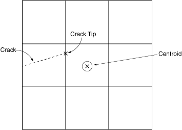
By default, the stress/strain computed at the element centroid ahead of the crack tip is used to determine if the damage initiation criterion is satisfied and to determine the crack propagation direction. See Figure 10.7.1–7.
| Input File Usage: | *DAMAGE INITIATION, POSITION=CENTROID (default) |
| Abaqus/CAE Usage: | Property module: material editor: Mechanical |
With a sufficiently refined mesh, the centroidal approximation is accurate and economical. However, if the finite element mesh in the vicinity of the crack tip is coarse relative to the gradients in the stress/strain fields, the default centroidal approximation may not be sufficient. In such cases you can use the stress/strain extrapolated to the crack tip to determine if the damage initiation criterion is satisfied and to determine the crack propagation direction. See Figure 10.7.1–7.
| Input File Usage: | *DAMAGE INITIATION, POSITION=CRACKTIP |
| Abaqus/CAE Usage: | Property module: material editor: Mechanical |
You can also choose to combine the two previous alternatives: you can use the stress/strain values extrapolated to the crack tip to determine if the damage initiation criterion is satisfied, and you can use the stress/strain values at the element centroid to determine the crack propagation direction.
| Input File Usage: | *DAMAGE INITIATION, POSITION=COMBINED |
| Abaqus/CAE Usage: | Property module: material editor: Mechanical |
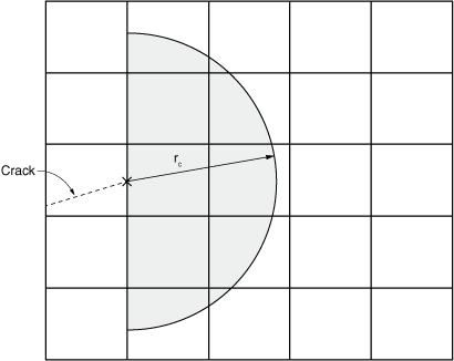
The three options for evaluating the stress and strain fields discussed above are local calculations in the sense that the evaluated fields are local to the single element ahead of the crack tip. In the case of coarse and/or unstructured meshes a nonlocal averaging of the stress and strain fields ahead of the crack tip can lead to a more accurate evaluation of those fields, which can improve the accuracy of the computed propagation directions. See Figure 10.7.1–8.
| Input File Usage: | *DAMAGE INITIATION, POSITION=NONLOCAL |
| Abaqus/CAE Usage: | Nonlocal averaging of the stress/strain fields ahead of the crack tip is not supported in Abaqus/CAE. |
To control the range of elements used for nonlocal averaging in the crack direction calculations, you can specify a radius, ![]() , within which the elements ahead of the crack tip are included. The default radius is three times the typical element characteristic length in the enriched region.
, within which the elements ahead of the crack tip are included. The default radius is three times the typical element characteristic length in the enriched region.
| Input File Usage: | *DAMAGE INITIATION, R CRACK DIRECTION= |
| Abaqus/CAE Usage: | Specifying the range of the model for nonlocal averaging is not supported in Abaqus/CAE. |
To further improve the nonlocal averaging, you can request an initial smoothing of the stress/strain fields ahead of the crack. In this case Abaqus/Standard averages the field values to element nodes and then interpolates the smoothed fields to the integration points. Once smoothing is complete, the nonlocal averaging is applied. No smoothing is applied by default.
| Input File Usage: | Use one of the following options: |
*DAMAGE INITIATION, SMOOTHING=NONE (default) *DAMAGE INITIATION, SMOOTHING=NODAL |
| Abaqus/CAE Usage: | Smoothing the stress/strain fields before averaging is not supported in Abaqus/CAE. |
Abaqus/Standard offers a number of weighting schemes for field smoothing that provide additional control over nonlocal averaging. For example, you may want to give a higher weighting to elements close to the crack tip. You can specify a weight function, ![]() , to compute the average stress/strain based on the distance from the element integration points to the crack tip,
, to compute the average stress/strain based on the distance from the element integration points to the crack tip, ![]() . By default, a uniform weighting is applied to all elements used for averaging; alternatively, you can use a Gaussian function or a cubic spline function. You can also define a weight function with a user subroutine.
. By default, a uniform weighting is applied to all elements used for averaging; alternatively, you can use a Gaussian function or a cubic spline function. You can also define a weight function with a user subroutine.
The Gaussian function is represented by:
![]()
| Input File Usage: | Use one of the following options: |
*DAMAGE INITIATION, WEIGHTING METHOD=UNIFORM (default) *DAMAGE INITIATION, WEIGHTING METHOD=GAUSS *DAMAGE INITIATION, WEIGHTING METHOD=CUBIC SPLINE *DAMAGE INITIATION, WEIGHTING METHOD=USER |
| Abaqus/CAE Usage: | Specifying a weighting scheme for nonlocal averaging is not supported in Abaqus/CAE. |
The damage evolution law describes the rate at which the cohesive stiffness is degraded once the corresponding initiation criterion is reached. The general framework for describing the evolution of damage is conceptually similar to that used for damage evolution in surface-based cohesive behavior (“Surface-based cohesive behavior,” Section 37.1.10).
A scalar damage variable, D, represents the averaged overall damage at the intersection between the crack surfaces and the edges of cracked elements. It initially has a value of 0. If damage evolution is modeled, D monotonically evolves from 0 to 1 upon further loading after the initiation of damage. The normal and shear stress components are affected by the damage according to
![]()
![]()
![]()
To describe the evolution of damage under a combination of normal and shear separations across the interface, an effective separation is defined as
![]()
| Input File Usage: | Use the following option to specify a damage evolution law: |
*DAMAGE EVOLUTION |
| Abaqus/CAE Usage: | Property module: material editor: Mechanical |
A separate damage evolution law should be specified for each damage initiation criterion defined in user subroutine UDMGINI. Each combination of a damage initiation criterion and a corresponding damage evolution law is referred to as a failure mechanism. Damage will accumulate for only one failure mechanism per element, corresponding to the mechanism whose damage initiation criterion was achieved first.
| Input File Usage: | Use the following options to specify damage evolution laws for multiple user-defined damage initiation criteria: |
*DAMAGE INITIATION, CRITERION=USER, FAILURE MECHANISMS= |
| Abaqus/CAE Usage: | Defining a user-defined damage initiation criterion is not supported in Abaqus/CAE. |
Models exhibiting various forms of softening behavior and stiffness degradation often lead to severe convergence difficulties in Abaqus/Standard. Viscous regularization of the constitutive equations defining cohesive behavior in an enriched element can be used to overcome some of these convergence difficulties. Viscous regularization damping causes the tangent stiffness matrix to be positive definite for sufficiently small time increments.
The approximate amount of energy associated with viscous regularization over the whole model is available using output variable ALLVD.
| Input File Usage: | Use the following option to specify viscous regularization: |
*DAMAGE STABILIZATION |
| Abaqus/CAE Usage: | Property module: material editor: Mechanical |
The formulae and laws that govern the behavior of fluid flow within the XFEM-based cracked element surfaces are very similar to those used for fluid flow within the cohesive element gap (“Defining the constitutive response of fluid within the cohesive element gap,” Section 32.5.7). The similarities extend to the traction-separation model, damage initiation criteria, damage evolution law, and the fluid flow behavior. The fluid constitutive response comprises the tangential flow within the cracked element surfaces and the normal flow across the cracked element surfaces due to caking or fouling effects in the enriched elements.
The tangential flow within the cracked element surfaces can be modeled with either a Newtonian or power-law model. By default, there is no tangential flow of pore fluid within the cracked element surfaces. To allow tangential flow, define a gap flow property in conjunction with the pore fluid material definition.
In the case of a Newtonian fluid the volume flow rate density vector is given by the expression
![]()
Abaqus defines the tangential permeability, or the resistance to flow, according to Reynold's equation:
![]()
In the case of a power law fluid the constitutive relation is defined as
![]()
By default, the gap between the cracked element surfaces has an initial opening of 0.002 in both a Newtonian fluid and a power law fluid. However, you can specify this opening directly.
| Input File Usage: | Use the following option to define the tangential flow in a Newtonian fluid: |
*GAP FLOW, TYPE=NEWTONIAN, KMAX Use the following option to define the tangential flow in a power law fluid: *GAP FLOW, TYPE=POWER LAW Use the following option to define the initial gap opening directly: *SECTION CONTROLS, INITIAL GAP OPENING |
| Abaqus/CAE Usage: | Use the following option to define the tangential flow in a Newtonian fluid: |
Property module: material editor: Other Use the following option to define the tangential flow in a power law fluid: Property module: material editor: Other An initial gap opening is not supported in Abaqus/CAE. |
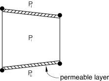
You can permit normal flow by defining a fluid leakoff coefficient for the pore fluid material. This coefficient defines a pressure-flow relationship between the phantom nodes located at the cracked element edges and cracked element surfaces. The fluid leakoff coefficients can be interpreted as the permeability of a finite layer of material on the cracked element surfaces, as shown in Figure 10.7.1–9.
The normal flow is defined as![]()
![]()
Alternatively, you can use user subroutine UFLUIDLEAKOFF to define more complex leakoff behavior, including the ability to define a time accumulated resistance, or fouling, through the use of solution-dependent state variables.
| Input File Usage: | Use the following option to define the leakoff coefficients: |
*FLUID LEAKOFF Use the following option to define leakoff coefficients as functions of temperature and field variables: *FLUID LEAKOFF, DEPENDENCIES Use the following option to define more complex leakoff behavior in user subroutine UFLUIDLEAKOFF: *FLUID LEAKOFF, USER |
| Abaqus/CAE Usage: | Use the following option to define the leakoff coefficients: |
Property module: material editor: Other Use the following option to define leakoff coefficients as functions of temperature and field variables: Property module: material editor: Other Use the following option to define more complex leakoff behavior in user subroutine UFLUIDLEAKOFF: Property module: material editor: Other |
The formulae and laws that govern the behavior of the XFEM-based linear elastic fracture mechanics approach for crack propagation analysis are very similar to those used for modeling delamination along a known and partially bonded surface (see “Crack propagation analysis,” Section 11.4.3), where the strain energy release rate at the crack tip is calculated based on the modified Virtual Crack Closure Technique (VCCT). However, unlike this method, the XFEM-based LEFM approach can be used to simulate crack propagation along an arbitrary, solution-dependent path in the bulk material with or without an initial crack. You complete the definition of the crack propagation capability by defining a fracture-based surface behavior and specifying the fracture criterion in enriched elements.
By definition, the XFEM-based LEFM approach inherently requires the presence of a crack in the model since it is based on the principles of linear elastic fracture mechanics. The crack can be pre-existing, or it can nucleate during the analysis. If there is no pre-existing crack for a given enriched region, the XFEM-based LEFM approach is not activated until a crack nucleates. The crack nucleation is governed by one of the six built-in stress- or strain-based crack initiation criteria or a user-defined crack initiation criterion discussed in “Crack initiation and direction of crack extension,” above. After a crack is nucleated in an enriched region, subsequent propagation of the crack is governed by the XFEM-based LEFM criterion.
| Input File Usage: | Use the following option to specify the crack nucleation criterion as part of the material definition when there is no pre-existing crack in an enriched region: |
*DAMAGE INITIATION, TOLERANCE= |
| Abaqus/CAE Usage: | Property module: material editor: Mechanical: Damage for Traction Separation Laws: Quade Damage, Maxe Damage, Quads Damage, Maxs Damage, Maxpe Damage, or Maxps Damage: |
If there is a pre-existing crack in an enriched region, the crack extends after an equilibrium increment when the fracture criterion, f, reaches the value 1.0 within a given tolerance:
![]()
| Input File Usage: | Use both of the following options: |
*SURFACE BEHAVIOR *FRACTURE CRITERION, TOLERANCE= |
| Abaqus/CAE Usage: | Interaction module: Interaction |
You must specify the crack propagation direction when the fracture criterion is satisfied. The crack can extend at a direction normal to the direction of the maximum tangential stress, orthogonal to the element local 1-direction (see “Conventions,” Section 1.2.2), or orthogonal to the element local 2-direction. By default, the crack propagates normal to the direction of the maximum tangential stress.
| Input File Usage: | Use one of the following options to specify the crack direction when the fracture criterion is satisfied: |
*FRACTURE CRITERION, NORMAL DIRECTION=MTS (default) *FRACTURE CRITERION, NORMAL DIRECTION=1 *FRACTURE CRITERION, NORMAL DIRECTION=2 |
| Abaqus/CAE Usage: | Interaction module: contact property editor: Mechanical |
Abaqus provides three common mode-mix formulae for computing the equivalent fracture energy release rate ![]() : the BK law, the power law, and the Reeder law models. The choice of model is not always clear in any given analysis; an appropriate model is best selected empirically.
: the BK law, the power law, and the Reeder law models. The choice of model is not always clear in any given analysis; an appropriate model is best selected empirically.
The BK law model is described in Benzeggagh and Kenane (1996) by the following formula:
![]()
To define this model, you must provide ![]() and
and ![]() . This model provides a power law relationship combining energy release rates in Mode I, Mode II, and Mode III into a single scalar fracture criterion.
. This model provides a power law relationship combining energy release rates in Mode I, Mode II, and Mode III into a single scalar fracture criterion.
| Input File Usage: | *FRACTURE CRITERION, TYPE=VCCT, MIXED MODE BEHAVIOR=BK |
| Abaqus/CAE Usage: | Interaction module: contact property editor: Mechanical |
The power law model is described in Wu and Reuter (1965) by the following formula:
![]()
To define this model, you must provide ![]() and
and ![]() .
.
| Input File Usage: | *FRACTURE CRITERION, TYPE=VCCT, MIXED MODE BEHAVIOR=POWER |
| Abaqus/CAE Usage: | Interaction module: contact property editor: Mechanical |
The Reeder law model is described in Reeder et al. (2002) by the following formula:
![]()
![]()
To define this model, you must provide ![]() and
and ![]() . The Reeder law is best applied when
. The Reeder law is best applied when ![]() ; when
; when ![]() , the Reeder law reduces to the BK law. The Reeder law applies only to three-dimensional problems.
, the Reeder law reduces to the BK law. The Reeder law applies only to three-dimensional problems.
| Input File Usage: | *FRACTURE CRITERION, TYPE=VCCT, MIXED MODE BEHAVIOR=REEDER |
| Abaqus/CAE Usage: | Interaction module: contact property editor: Mechanical |
You can define a VCCT criterion with varying energy release rates by specifying the critical energy release rates at the nodes.
If you indicate that the nodal critical energy rates will be specified, any constant critical energy release rates you specify are ignored and the critical energy release rates are interpolated from the nodes. The critical energy release rates must be defined at all nodes in the enriched region.
| Input File Usage: | Use both of the following options: |
*FRACTURE CRITERION, TYPE=VCCT, NODAL ENERGY RATE *NODAL ENERGY RATE |
| Abaqus/CAE Usage: | Defining a VCCT criterion with varying energy release rates is not supported in Abaqus/CAE. |
The formulae and laws governing the behavior of the enhanced VCCT criterion are very similar to those used for the VCCT criterion. However, unlike the VCCT criterion, the onset and growth of a crack can be controlled by two different critical fracture energy release rates: ![]() and
and ![]() . In a general case involving Mode I, II, and III fracture, when the fracture criterion is satisfied; i.e,
. In a general case involving Mode I, II, and III fracture, when the fracture criterion is satisfied; i.e,
![]()
| Input File Usage: | Use both of the following options: |
*SURFACE BEHAVIOR *FRACTURE CRITERION, TYPE=ENHANCED VCCT |
| Abaqus/CAE Usage: | Specifying the enhanced VCCT criterion is not supported in Abaqus/CAE. |
If you specify the low-cycle fatigue criterion, progressive crack growth at the enriched elements subjected to sub-critical cyclic loading can be simulated. This criterion can be used only in a low-cycle fatigue analysis using the direct cyclic approach (“Low-cycle fatigue analysis using the direct cyclic approach,” Section 6.2.7). A low-cycle fatigue step can be the only step, can follow a general static step, or can be followed by a general static step. You can include multiple low-cycle fatigue analysis steps in a single analysis. If you perform a fatigue analysis in a model without a pre-existing crack, you must precede the fatigue step with a static step that nucleates a crack, as discussed in “Crack nucleation and direction of crack extension.”
The onset and fatigue crack growth are characterized by using the Paris law, which relates the relative fracture energy release rate to crack growth rates as illustrated in Figure 10.7.1–4. The fracture energy release rates at the crack tips in the enriched elements are calculated based on the above mentioned VCCT technique.
The Paris regime is bounded by the energy release rate threshold, ![]() , below which there is no consideration of fatigue crack initiation or growth, and the energy release rate upper limit,
, below which there is no consideration of fatigue crack initiation or growth, and the energy release rate upper limit, ![]() , above which the fatigue crack will grow at an accelerated rate.
, above which the fatigue crack will grow at an accelerated rate. ![]() is the critical equivalent strain energy release rate calculated based on the user-specified mode-mix criterion and the fracture strength of the bulk material. The formulae for calculating
is the critical equivalent strain energy release rate calculated based on the user-specified mode-mix criterion and the fracture strength of the bulk material. The formulae for calculating ![]() have been provided above for different mixed mode fracture criteria. You can specify the ratio of
have been provided above for different mixed mode fracture criteria. You can specify the ratio of ![]() over
over ![]() and the ratio of
and the ratio of ![]() over
over ![]() . The default values are
. The default values are ![]() and
and ![]() .
.
| Input File Usage: | Use both of the following options: |
*SURFACE BEHAVIOR *FRACTURE CRITERION, TYPE=FATIGUE |
| Abaqus/CAE Usage: | Specifying a low-cycle fatigue criterion is not supported in Abaqus/CAE. |
The onset of fatigue crack growth refers to the beginning of fatigue crack growth at the crack tip in the enriched elements. In a low-cycle fatigue analysis the onset of the fatigue crack growth criterion is characterized by ![]() , which is the relative fracture energy release rate when the structure is loaded between its maximum and minimum values. The fatigue crack growth initiation criterion is defined as
, which is the relative fracture energy release rate when the structure is loaded between its maximum and minimum values. The fatigue crack growth initiation criterion is defined as
![]()
Once the onset of the fatigue crack growth criterion is satisfied at the enriched element, the crack growth rate, ![]() , can be calculated based on the relative fracture energy release rate,
, can be calculated based on the relative fracture energy release rate, ![]() . The rate of the crack growth per cycle is given by the Paris law if
. The rate of the crack growth per cycle is given by the Paris law if ![]()
![]()
At the end of cycle ![]() , Abaqus/Standard extends the crack length,
, Abaqus/Standard extends the crack length, ![]() , from the current cycle forward over an incremental number of cycles,
, from the current cycle forward over an incremental number of cycles, ![]() to
to ![]() by fracturing at least one enriched element ahead of the crack tips. Given the material constants
by fracturing at least one enriched element ahead of the crack tips. Given the material constants ![]() and
and ![]() , combined with the known element length and the likely crack propagation direction
, combined with the known element length and the likely crack propagation direction ![]() at the enriched elements ahead of the crack tips, the number of cycles necessary to fail each enriched element ahead of the crack tip can be calculated as
at the enriched elements ahead of the crack tips, the number of cycles necessary to fail each enriched element ahead of the crack tip can be calculated as ![]() , where j represents the enriched element ahead of the
, where j represents the enriched element ahead of the ![]() th crack tip. The analysis is set up to advance the crack by at least one enriched element after the loading cycle is stabilized. The element with the fewest cycles is identified to be fractured, and its
th crack tip. The analysis is set up to advance the crack by at least one enriched element after the loading cycle is stabilized. The element with the fewest cycles is identified to be fractured, and its ![]() is represented as the number of cycles to grow the crack equal to its element length,
is represented as the number of cycles to grow the crack equal to its element length, ![]() . The most critical element is completely fractured with a zero constraint and a zero stiffness at the end of the stabilized cycle. As the enriched element is fractured, the load is redistributed and a new relative fracture energy release rate must be calculated for the enriched elements ahead of the crack tips for the next cycle. This capability allows at least one enriched element ahead of the crack tips to be fractured completely after each stabilized cycle and precisely accounts for the number of cycles needed to cause fatigue crack growth over that length.
. The most critical element is completely fractured with a zero constraint and a zero stiffness at the end of the stabilized cycle. As the enriched element is fractured, the load is redistributed and a new relative fracture energy release rate must be calculated for the enriched elements ahead of the crack tips for the next cycle. This capability allows at least one enriched element ahead of the crack tips to be fractured completely after each stabilized cycle and precisely accounts for the number of cycles needed to cause fatigue crack growth over that length.
If ![]() , the enriched elements ahead of the crack tips will be fractured by increasing the cycle number count,
, the enriched elements ahead of the crack tips will be fractured by increasing the cycle number count, ![]() , by one only.
, by one only.
For information on how to accelerate the low-cycle fatigue analysis and to provide a smooth solution for the crack front, see “Controlling the accuracy of damage extrapolation at the interface elements and at the enriched elements” in “Low-cycle fatigue analysis using the direct cyclic approach,” Section 6.2.7.
The simulation of structures with unstable propagating cracks is challenging and difficult. Nonconvergent behavior may occur from time to time. Localized damping is included for the XFEM-based LEFM approach by using the viscous regularization technique. Viscous regularization damping causes the tangent stiffness matrix of the softening material to be positive for sufficiently small time increments.
| Input File Usage: | Use one of the following options |
*FRACTURE CRITERION, TYPE=VCCT, VISCOSITY= *FRACTURE CRITERION, TYPE=ENHANCED VCCT, VISCOSITY= |
| Abaqus/CAE Usage: | Interaction module: contact property editor: Mechanical |
When an element is cut by a crack during the analysis, a XFEM-based crack surface is generated during the analysis (see “Defining a crack surface,” above). A distributed pressure load can be applied to the cracked element surfaces.
| Input File Usage: | Use the following option to define a distributed pressure load to a crack surface: |
*DSLOAD surface name, P or PNU, magnitude |
| Abaqus/CAE Usage: | An XFEM-based crack surface is not supported in Abaqus/CAE. |
Because the mesh is not required to conform to the geometric discontinuities, the initial location of a pre-existing crack must be specified in the model. The level set method is provided for this purpose. Two signed distance functions per node are generally required to describe a crack geometry. The first describes the crack surface, while the second is used to construct an orthogonal surface so that the intersection of the two surfaces gives the crack front (see “Initial conditions in Abaqus/Standard and Abaqus/Explicit,” Section 34.2.1).
The first signed distance function must be either greater or less than zero and cannot be equal to zero. If an initial crack has to be defined at the boundaries of an element, a very small positive or negative value for the first signed distance function must be specified.
| Input File Usage: | Use the following option to specify the initial location of an enriched feature: |
*INITIAL CONDITIONS, TYPE=ENRICHMENT |
| Abaqus/CAE Usage: | Interaction module: crack editor: Crack location: Select: select region |
The crack propagation capability can be activated or deactivated within the step definition.
| Input File Usage: | Use the following option to activate the crack propagation capability within the step definition: |
*ENRICHMENT ACTIVATION, NAME=name, ACTIVATE=ON (default) Use the following option to deactivate the crack propagation capability within the step definition: *ENRICHMENT ACTIVATION, NAME=name, ACTIVATE=OFF Use the following option to deactivate the crack propagation capability automatically once all the pre-existing cracks (or if there are no pre-existing cracks, all the allowable newly nucleated cracks) have propagated through the boundary of the given enriched feature within the step definition: *ENRICHMENT ACTIVATION, NAME=name, ACTIVATE=AUTO OFF |
| Abaqus/CAE Usage: | To modify the status of the crack propagation capability in a step, you must first create an XFEM crack growth interaction: |
Interaction module: Create Interaction: select initial step: XFEM Crack Growth: select crack: Interaction manager: select interaction in step: Edit: toggle on/off Allow crack growth in this step |
When you evaluate the contour integrals using the conventional finite element method (“Contour integral evaluation,” Section 11.4.2), you must define the crack front explicitly and specify the virtual crack extension direction in addition to matching the mesh to the cracked geometry. Detailed focused meshes are generally required and obtaining accurate contour integral results for a crack in a three-dimensional curved surface can be cumbersome. The extended finite element in conjunction with the level set method alleviates these shortcomings. The adequate singular asymptotic fields and the discontinuity are ensured by the special enrichment functions in conjunction with additional degrees of freedom. In addition, the crack front and the virtual crack extension direction are determined automatically by the level set signed distance functions.
| Input File Usage: | Use the following option to obtain contour integral for a named enriched feature with the extended finite element method: |
*CONTOUR INTEGRAL, XFEM, CRACK NAME=name |
| Abaqus/CAE Usage: | Step module: history output request editor: Domain: Crack: crack name |
Although XFEM has alleviated the shortcomings associated with refining the mesh in the neighborhood of the crack front due to the added asymptotic fields, you must generate a sufficient number of elements around the crack front to obtain path-independent contours. The group of elements within a small radius from the crack front are enriched and become involved in the contour integral calculations. The default enrichment radius is three times the typical element characteristic length in the enriched area. You must include the elements inside the enrichment radius in the element set used to define the enriched region.
| Input File Usage: | Use the following option to specify an enrichment radius: |
*ENRICHMENT, ENRICHMENT RADIUS |
| Abaqus/CAE Usage: | Interaction module: crack editor: Enrichment radius: Analysis default or Specify |
Modeling discontinuities as an enriched feature can be performed using any of the following:
static analysis (see “Static stress analysis,” Section 6.2.2);
implicit dynamic analysis (see “Implicit dynamic analysis using direct integration,” Section 6.3.2); or
low-cycle fatigue analysis using the direct cyclic approach (“Low-cycle fatigue analysis using the direct cyclic approach,” Section 6.2.7).
geostatic stress field analysis (see “Geostatic stress state,” Section 6.8.2); or
coupled pore fluid diffusion/stress analysis (see “Coupled pore fluid diffusion and stress analysis,” Section 6.8.1).
Initial conditions to identify initial boundaries or interfaces of an enriched feature can be specified (see “Initial conditions in Abaqus/Standard and Abaqus/Explicit,” Section 34.2.1).
Boundary conditions can be applied to any of the displacement or pore pressure degrees of freedom (see “Boundary conditions in Abaqus/Standard and Abaqus/Explicit,” Section 34.3.1).
The following types of loading can be prescribed in a model with an enriched feature:
Concentrated nodal forces can be applied to the displacement degrees of freedom (1–3) or the pore pressure degree of freedom (8); see “Concentrated loads,” Section 34.4.2.
Distributed pressure forces or body forces can be applied; see “Distributed loads,” Section 34.4.3. The distributed load types available with particular elements are described in Part VI, “Elements.”
The following predefined fields can be specified in a model with an enriched feature, as described in “Predefined fields,” Section 34.6.1:
Nodal temperatures (although temperature is not a degree of freedom in stress/displacement elements). The specified temperature affects temperature-dependent critical stress and strain failure criteria.
The values of user-defined field variables. The specified value affects field-variable-dependent material properties.
Any of the mechanical constitutive models in Abaqus/Standard, including user-defined materials (defined using user subroutine “UMAT,” Section 1.1.44 of the Abaqus User Subroutines Reference Guide) can be used to model the mechanical behavior of the enriched element in a crack propagation analysis. See Part V, “Materials.” The inelastic definition at a material point must be used in conjunction with the linear elastic material model (“Linear elastic behavior,” Section 22.2.1) or the hypoelastic material model (“Hypoelastic behavior,” Section 22.4.1). Only isotropic elastic materials are supported when evaluating the contour integral for a stationary crack.
Only first-order solid continuum stress/displacement elements, first-order displacement/pore pressure solid continuum elements, and second-order stress/displacement tetrahedron elements can be associated with an enriched feature. For propagating cracks these include bilinear plane strain and plane stress elements, bilinear axisymmetric elements, linear brick elements, linear tetrahedron elements, and second-order tetrahedron elements. For stationary cracks, these include linear brick elements, linear tetrahedron elements, and second-order tetrahedron elements.
For an incompatible mode element, Abaqus/Standard discards the contribution due to the incompatible deformation mode immediately after the element is fractured under a tensile loading. Therefore, the stress level at the cracked element may not return completely to its originally unloaded state even when this cracked element is unloaded completely and the contact of the cracked element surfaces is reestablished.
In addition to the standard output identifiers available in Abaqus (“Abaqus/Standard output variable identifiers,” Section 4.2.1), the following nodal, whole element, and surface variables have special meaning for a model with an enriched feature.
PHILSM | Signed distance function to describe the crack surface. |
PSILSM | Signed distance function to describe the initial crack front. |
STATUSXFEM | Status of the enriched element. (The status of an enriched element is 1.0 if the element is completely cracked and 0.0 if the element contains no crack. If the element is partially cracked, the value of STATUSXFEM lies between 1.0 and 0.0.) |
ENRRTXFEM | All components of strain energy release rate when linear elastic fracture mechanics with the extended finite element method is used. |
LOADSXFEM | Distributed pressure loads applied to the crack surface. |
GFVRXFEM | Gap fluid volume rate of the enriched element. |
CRDCUTXFEM | Crack midpoint coordinates at the element edges of the enriched element. |
PFOPENXFEM | Fracture opening of the enriched element. |
PFOPENXFEMCOMP | Fracture opening at the element edges of the enriched element. |
PORPRES | Fluid pressure of the enriched element. |
PORPRESCOMP | Fluid pressure at the element edges of the enriched element. |
LEAKVRTXFEM | Leak-off flow rate at the top of the enriched element. |
LEAKVRBXFEM | Leak-off flow rate at the bottom of the enriched element. |
ALEAKVRTXFEM | Accumulated leak-off flow volume at the top of the enriched element. |
ALEAKVRBXFEM | Accumulated leak-off flow volume at the bottom of the enriched element. |
CRKDISP | Crack opening and relative tangential motions on cracked surfaces in enriched elements. |
CSDMG | Damage variable on cracked surfaces in enriched elements. |
CRKSTRESS | Remaining residual pressure and tangential shear stresses on cracked surfaces in enriched elements. |
GFVR | Fluid volume rate within the cracked surfaces in the enriched element. |
PORPRES | Pore pressure within the cracked surfaces in the enriched element. |
PORPRESURF | Pore pressure on the cracked surfaces in the enriched element. |
LEAKVR | Leak-off flow rate on the cracked surfaces in the enriched element. |
ALEAKVR | Accumulated leak-off flow volume on the cracked surfaces in the enriched element. |
When the pore pressure degrees of freedom are activated in the enriched elements, matrices are unsymmetric; therefore, unsymmetric matrix storage and solution may be needed to improve convergence (see “Matrix storage and solution scheme in Abaqus/Standard” in “Defining an analysis,” Section 6.1.2).
A crack can be visualized through the iso-surface for the signed distance function PHILSM.
If a crack cuts through a very tiny corner of an enriched element, the displacements along the crack front in the enriched element may be distorted in rare cases in the Visualization module of Abaqus/CAE (Abaqus/Viewer) when displaying the contours. The distortion, however, is not present when viewing only the deformed shape.
When an element is cut through by a crack, the cracked element splits into two parts, each part formed by a real domain and a phantom domain, as illustrated in Figure 10.7.1–2. Contour plot integration point values for cracked elements consider contributions from only the real domains in both parts of the cracked elements. However, when you probe cracked elements, only the contribution from the part of the elements containing the real domain ![]() and the phantom domain
and the phantom domain ![]() is reported.
is reported.
When evaluating the contour integrals in a stationary crack, additional integration stations are introduced internally in the elements enriched with singular asymptotic crack-tip fields. However, visualization of the element output variables in those additional integration points is not supported in the Visualization module of Abaqus/CAE (Abaqus/Viewer).
The following limitations exist with an enriched feature:
An enriched element cannot be intersected by more than one crack.
A crack is not allowed to turn more than 90° in one increment during an analysis.
Only asymptotic crack-tip fields in an isotropic elastic material are considered for a stationary crack.
Adaptive remeshing is not supported.
Composite solid elements are not supported.
Import analysis is not supported.
The following is an example of modeling crack propagation with the XFEM-based cohesive segments method:
*HEADING
...
*NODE, NSET=ALL
...
*ELEMENT, TYPE=C3D8, ELSET=REGULAR
*ELEMENT, TYPE=C3D8, ELSET=ENRICHED
...
*SOLID SECTION, MATERIAL=STEEL1, ELSET=REGULAR
*SOLID SECTION, MATERIAL=STEEL12, ELSET=ENRICHED

*ENRICHMENT, TYPE=PROPAGATION CRACK, ELSET=ENRICHED,
NAME=ENRICHMENT, INTERACTION=INTERACTION
*SURFACE, TYPE=XFEM, NAME=SURF_NAME
Data lines to specify the names of enriched features
*MATERIAL, NAME=STEEL1
...
*MATERIAL, NAME=STEEL2
*DAMAGE INITIATION, CRITERION=MAXPS, TOLERANCE=0.05
*DAMAGE EVOLUTION, TYPE=ENERGY
Data lines to specify the failure mechanism
...
*SURFACE INTERACTION, NAME=INTERACTION
*SURFACE BEHAVIOR
Data lines to specify the contact of cracked element surfaces
...
*STEP
*STATIC
...
*END STEP
*STEP
*STATIC
...

*ENRICHMENT ACTIVATION, TYPE=PROPAGATION CRACK,
NAME=ENRICHMENT, ACTIVATE=OFF
...
*END STEP
The following is an example of modeling crack propagation with the XFEM-based LEFM approach:
*HEADING
...
*NODE, NSET=ALL
...
*ELEMENT, TYPE=C3D8, ELSET=REGULAR
*ELEMENT, TYPE=C3D8, ELSET=ENRICHED
...
*SOLID SECTION, MATERIAL=STEEL1, ELSET=REGULAR
*SOLID SECTION, MATERIAL=STEEL12, ELSET=ENRICHED

*ENRICHMENT, TYPE=PROPAGATION CRACK, ELSET=ENRICHED,
NAME=ENRICHMENT, INTERACTION=INTERACTION
*MATERIAL, NAME=STEEL1
...
*MATERIAL, NAME=STEEL2
*DAMAGE INITIATION, CRITERION=MAXPS, TOLERANCE=0.05
Data lines to specify the crack nucleation mechanism
...
*SURFACE INTERACTION, NAME=INTERACTION
*SURFACE BEHAVIOR
*FRACTURE CRITERION, TYPE=VCCT, TOLERANCE=0.05,VISCOSITY=0.00001
Data lines to specify the crack propagation criterion
...
*END STEP
The following is an example of calculating contour integrals in stationary cracks with the extended finite element method:
*HEADING
...
*NODE, NSET=ALL
...
*ELEMENT, TYPE=C3D8, ELSET=REGULAR
*ELEMENT, TYPE=C3D8, ELSET=ENRICHED
...
*SOLID SECTION, MATERIAL=STEEL1, ELSET=REGULAR
*SOLID SECTION, MATERIAL=STEEL12, ELSET=ENRICHED

*ENRICHMENT, TYPE=STATIONARY CRACK, ELSET=ENRICHED,
NAME=ENRICHMENT, ENRICHMENT RADIUS
*MATERIAL, NAME=STEEL1
...
*MATERIAL, NAME=STEEL2
...
*STEP
*STATIC
...
*CONTOUR INTEGRAL, CRACK NAME=ENRICHMENT, XFEM
*END STEP
Belytschko, T., and T. Black, “Elastic Crack Growth in Finite Elements with Minimal Remeshing,” International Journal for Numerical Methods in Engineering, vol. 45, pp. 601–620, 1999.
Benzeggagh, M., and M. Kenane, “Measurement of Mixed-Mode Delamination Fracture Toughness of Unidirectional Glass/Epoxy Composites with Mixed-Mode Bending Apparatus,” Composite Science and Technology, vol. 56 439, 1996.
Elguedj, T., A. Gravouil, and A. Combescure, “Appropriate Extended Functions for X-FEM Simulation of Plastic Fracture Mechanics,” Computer Methods in Applied Mechanics and Engineering, vol. 195, pp. 501–515, 2006.
Melenk, J., and I. Babuska, “The Partition of Unity Finite Element Method: Basic Theory and Applications,” Computer Methods in Applied Mechanics and Engineering, vol. 39, pp. 289–314, 1996.
Reeder, J., S. Kyongchan, P. B. Chunchu, and D. R.. Ambur, “Postbuckling and Growth of Delaminations in Composite Plates Subjected to Axial Compression”43rd AIAA/ASME/ASCE/AHS/ASC Structures, Structural Dynamics, and Materials Conference, Denver, Colorado, vol. 1746, p. 10, 2002.
Remmers, J. J. C., R. de Borst, and A. Needleman, “The Simulation of Dynamic Crack Propagation using the Cohesive Segments Method,” Journal of the Mechanics and Physics of Solids, vol. 56, pp. 70–92, 2008.
Song, J. H., P. M. A. Areias, and T. Belytschko, “A Method for Dynamic Crack and Shear Band Propagation with Phantom Nodes,” International Journal for Numerical Methods in Engineering, vol. 67, pp. 868–893, 2006.
Sukumar, N., Z. Y. Huang, J.-H. Prevost, and Z. Suo, “Partition of Unity Enrichment for Bimaterial Interface Cracks,” International Journal for Numerical Methods in Engineering, vol. 59, pp. 1075–1102, 2004.
Sukumar, N., and J.-H. Prevost, “Modeling Quasi-Static Crack Growth with the Extended Finite Element Method Part I: Computer Implementation,” International Journal for Solids and Structures, vol. 40, pp. 7513–7537, 2003.
Wu, E. M., and R. C. Reuter Jr., “Crack Extension in Fiberglass Reinforced Plastics,” T and M Report, University of Illinois, vol. 275, 1965.