Products: Abaqus/Standard Abaqus/CAE
A direct-solution steady-state dynamic analysis:
is used to calculate the steady-state dynamic linearized response of a system to harmonic excitation;
is a linear perturbation procedure;
calculates the response directly in terms of the physical degrees of freedom of the model;
is an alternative to mode-based steady-state dynamic analysis, in which the response of the system is calculated on the basis of the eigenmodes;
is more expensive computationally than mode-based or subspace-based steady-state dynamics;
is more accurate than mode-based or subspace-based steady-state dynamics, in particular if significant frequency-dependent material damping or viscoelastic material behavior is present in the structure; and
is able to bias the excitation frequencies toward the approximate values that generate a response peak.
Steady-state dynamic analysis provides the steady-state amplitude and phase of the response of a system due to harmonic excitation at a given frequency. Usually such analysis is done as a frequency sweep by applying the loading at a series of different frequencies and recording the response; in Abaqus/Standard the direct-solution steady-state dynamic procedure conducts this frequency sweep. In a direct-solution steady-state analysis the steady-state harmonic response is calculated directly in terms of the physical degrees of freedom of the model using the mass, damping, and stiffness matrices of the system.
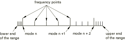
When defining a direct-solution steady-state dynamic step, you specify the frequency ranges of interest and the number of frequencies at which results are required in each range (including the bounding frequencies of the range). In addition, you can specify the type of frequency spacing (linear or logarithmic) to be used, as described below (“Selecting the frequency spacing”). Logarithmic frequency spacing is the default. Frequencies are given in cycles/time.
Those frequency points for which results are required can be spaced equally along the frequency axis (on a linear or a logarithmic scale), or they can be biased toward the ends of the user-defined frequency range by introducing a bias parameter (described below).
The direct-solution steady-state analysis procedure can be used in the following cases for which the eigenvalues cannot be extracted (and, thus, the mode-based steady-state dynamics procedures are not applicable):
for nonsymmetric stiffness;
when any form of damping other than modal damping must be included; and
when viscoelastic material properties must be taken into account.
While the response in this procedure is linear, the prior response can be nonlinear. Initial stress effects (stress stiffening) as well as load stiffness effects will be included in the steady-state dynamics response if nonlinear geometric effects (“General and linear perturbation procedures,” Section 6.1.3) were included in any general analysis step prior to the direct-solution steady-state dynamic procedure.
| Input File Usage: | *STEADY STATE DYNAMICS, DIRECT |
| Abaqus/CAE Usage: | Step module: Create Step: Linear perturbation: Steady-state dynamics, Direct |
If damping terms can be ignored, you can specify that a real, rather than a complex, system matrix be factored, which can significantly reduce computational time. Damping is discussed below.
| Input File Usage: | *STEADY STATE DYNAMICS, DIRECT, REAL ONLY |
| Abaqus/CAE Usage: | Step module: Create Step: Linear perturbation: Steady-state dynamics, Direct: Compute real response only |
Three types of frequency intervals are permitted for output from a direct-solution steady-state dynamic step. If an eigenvalue extraction step precedes the direct-solution steady-state dynamic step, you can select either the range or the eigenfrequency type of frequency interval; otherwise, only the range type can be used.
For the range type of frequency interval (the default), the specified frequency range of interest is divided using the user-defined number of points and the optional bias function.
| Input File Usage: | *STEADY STATE DYNAMICS, DIRECT, INTERVAL=RANGE |
| Abaqus/CAE Usage: | Step module: Create Step: Linear perturbation: Steady-state dynamics, Direct: toggle off Use eigenfrequencies to subdivide each frequency range |
If the direct-solution steady-state dynamic analysis is preceded by an eigenfrequency extraction step, you can select the eigenfrequency type of frequency interval. The following intervals then exist in each frequency range:
First interval: extends from the lower limit of the frequency range given to the first eigenfrequency in the range.
Intermediate intervals: extend from eigenfrequency to eigenfrequency.
Last interval: extends from the highest eigenfrequency in the range to the upper limit of the frequency range.
| Input File Usage: | *STEADY STATE DYNAMICS, DIRECT, INTERVAL=EIGENFREQUENCY |
| Abaqus/CAE Usage: | Step module: Create Step: Linear perturbation: Steady-state dynamics, Direct: Use eigenfrequencies to subdivide each frequency range |
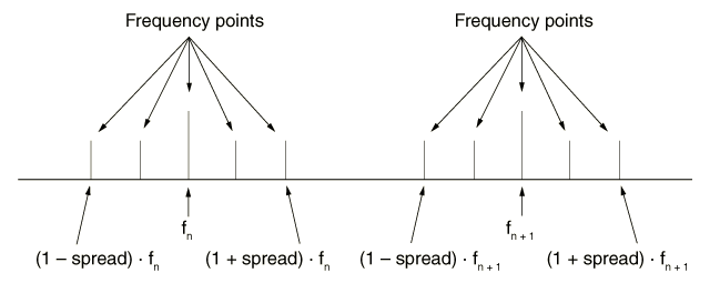
If the direct-solution steady-state dynamic analysis is preceded by an eigenfrequency extraction step, you can select the spread type of frequency interval. In this case intervals exist around each eigenfrequency in the frequency range. For each of the intervals the equally spaced frequencies at which results are calculated are determined using the user-defined number of points (which includes the bounding frequencies for the interval). The minimum number of frequency points is 3. If the user-defined value is less than 3 (or omitted), the default value of 3 points is assumed. Figure 6.3.4–2 illustrates the division of the frequency range for 5 calculation points.
The bias parameter is not supported with the spread type of frequency interval.
Figure 6.3.4–2 Division of range for the spread type of interval and 5 calculation points. ![]() and
and ![]() are eigenfrequencies of the system.
are eigenfrequencies of the system.
| Input File Usage: | *STEADY STATE DYNAMICS, DIRECT, INTERVAL=SPREAD lwr_freq, upr_freq, numpts, bias_param, freq_scale_factor, spread |
| Abaqus/CAE Usage: | You cannot specify frequency ranges by frequency spread in Abaqus/CAE. |
Two types of frequency spacing are permitted for a direct-solution steady-state dynamic step. For the logarithmic frequency spacing (the default), the specified frequency ranges of interest are divided using a logarithmic scale. Alternatively, a linear frequency spacing can be used if a linear scale is desired.
| Input File Usage: | Use either of the following options: |
*STEADY STATE DYNAMICS, DIRECT, FREQUENCY SCALE=LOGARITHMIC *STEADY STATE DYNAMICS, DIRECT, FREQUENCY SCALE=LINEAR |
| Abaqus/CAE Usage: | Step module: Create Step: Linear perturbation: Steady-state dynamics, Direct: Scale: Logarithmic or Linear |
You can request multiple frequency ranges or multiple single frequency points for a direct-solution steady-state dynamic step.
| Input File Usage: | *STEADY STATE DYNAMICS, DIRECT lwr_freq1, upr_freq1, numpts1, bias_param1, freq_scale_factor1 lwr_freq2, upr_freq2, numpts2, bias_param2, freq_scale_factor2 ... single_freq1 single_freq2 ... |
Repeat the data lines as often as necessary. |
| Abaqus/CAE Usage: | Step module: Create Step: Linear perturbation: Steady-state dynamics, Direct: Data: enter data in table, and add rows as necessary |
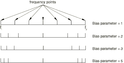
The bias parameter can be used to provide closer spacing of the results points either toward the middle or toward the ends of each frequency interval. Figure 6.3.4–3 shows a few examples of the effect of the bias parameter on the frequency spacing.
The bias formula used in direct-solution steady-state dynamics is
![]()
y
![]() ;
;
n
is the number of frequency points at which results are to be given;
k
is one such frequency point (![]() );
);
![]()
is the lower limit of the frequency range;
![]()
is the upper limit of the range;
![]()
is the frequency at which the kth results are given;
p
is the bias parameter value; and
![]()
is the frequency or the logarithm of the frequency, depending on the value chosen for the frequency scale.
The frequency scale factor can be used to scale frequency points. All the frequency points, except the lower and upper limit of the frequency range, are multiplied by this factor. This scale factor can be used only when the frequency interval is specified by using the system's eigenfrequencies (see “Specifying the frequency ranges by using the system's eigenfrequencies,” above).
If damping is absent, the response of a structure will be unbounded if the forcing frequency is equal to an eigenfrequency of the structure. To get quantitatively accurate results, especially near natural frequencies, accurate specification of damping properties is essential. The various damping options available are discussed in “Material damping,” Section 26.1.1.
In direct-solution steady-state dynamics damping can be created by the following:
dashpots (see “Dashpots,” Section 32.2.1),
“Rayleigh” damping associated with materials and elements (see “Material damping,” Section 26.1.1),
damping associated with acoustic elements (see “Acoustic medium,” Section 26.3.1; “Infinite elements,” Section 28.3.1; and “Acoustic and shock loads,” Section 34.4.6),
structural damping (see “Damping in dynamic analysis” in “Dynamic analysis procedures: overview,” Section 6.3.1), and
viscoelasticity included in the material definitions (see “Frequency domain viscoelasticity,” Section 22.7.2).
When a real-only system matrix is factored, all forms of damping are ignored, including quiet boundaries on infinite elements and nonreflecting boundaries on acoustic elements.
Abaqus/Standard automatically detects the contact nodes that are slipping due to velocity differences imposed by the motion of the reference frame or the transport velocity in prior steps. At those nodes the tangential degrees of freedom are not constrained and the effect of friction results in an unsymmetric contribution to the stiffness matrix. At other contact nodes the tangential degrees of freedom are constrained.
Friction at contact nodes at which a velocity differential is imposed can give rise to damping terms. There are two kinds of friction-induced damping effects. The first effect is caused by the friction forces stabilizing the vibrations in the direction perpendicular to the slip direction. This effect exists only in three-dimensional analysis. The second effect is caused by a velocity-dependent friction coefficient. If the friction coefficient decreases with velocity (which is usually the case), the effect is destabilizing and is also known as “negative damping.” For more details, see “Coulomb friction,” Section 5.2.3 of the Abaqus Theory Guide. Direct-solution steady-state dynamics analysis allows you to include these friction-induced contributions to the damping matrix.
| Input File Usage: | *STEADY STATE DYNAMICS, DIRECT, FRICTION DAMPING=YES |
| Abaqus/CAE Usage: | Step module: Create Step: Linear perturbation: Steady-state dynamics, Direct: Include friction-induced damping effects |
The base state is the current state of the model at the end of the last general analysis step prior to the steady-state dynamic step. If the first step of an analysis is a perturbation step, the base state is determined from the initial conditions (“Initial conditions in Abaqus/Standard and Abaqus/Explicit,” Section 34.2.1). Initial condition definitions that directly define solution variables, such as velocity, cannot be used in a steady-state dynamic analysis.
In a steady-state dynamic analysis the real and imaginary parts of any degree of freedom are either restrained or unrestrained simultaneously; it is physically impossible to have one part restrained and the other part unrestrained. Abaqus/Standard will automatically restrain both the real and imaginary parts of a degree of freedom even if only one part is prescribed specifically. The unspecified part will be assumed to have a perturbation magnitude of zero.
Boundary conditions can be applied to any of the displacement or rotation degrees of freedom (1–6) in a direct-solution steady-state analysis. See “Boundary conditions in Abaqus/Standard and Abaqus/Explicit,” Section 34.3.1. These boundary conditions will vary sinusoidally with time. You specify the real (in-phase) part of a boundary condition and the imaginary (out-of-phase) part of a boundary condition separately.
| Abaqus/CAE Usage: | Load module: boundary condition editor: real (in-phase) part + imaginary (out-of-phase) part i |
An amplitude definition can be used to specify the amplitude of a boundary condition as a function of frequency (“Amplitude curves,” Section 34.1.2).
| Input File Usage: | Use both of the following options: |
*AMPLITUDE, NAME=name *BOUNDARY, REAL or IMAGINARY, AMPLITUDE=name |
| Abaqus/CAE Usage: | Load or Interaction module: Create Amplitude: Name: name |
Load module: boundary condition editor: real (in-phase) part + imaginary (out-of-phase) part i: Amplitude: name |
The following loads can be prescribed in a steady-state dynamic analysis:
Concentrated nodal forces can be applied to the displacement degrees of freedom (1–6); see “Concentrated loads,” Section 34.4.2.
Distributed pressure forces or body forces can be applied; see “Distributed loads,” Section 34.4.3. The distributed load types available with particular elements are described in Part VI, “Elements.”
Incident wave loads can be applied; see “Acoustic and shock loads,” Section 34.4.6.
Coriolis distributed loading adds an imaginary antisymmetric contribution to the overall system of equations. This contribution is currently accounted for in solid and truss elements only and is activated by using the unsymmetric matrix storage and solution scheme for the step (“Defining an analysis,” Section 6.1.2).
Incident wave loads can be used to model sound waves from distinct planar or spherical sources or from diffuse fields.
Fluid flux loading cannot be used in a steady-state dynamic analysis.
| Abaqus/CAE Usage: | Load module: load editor: real (in-phase) part + imaginary (out-of-phase) part i |
An amplitude definition can be used to specify the amplitude of a load as a function of frequency (“Amplitude curves,” Section 34.1.2).
| Input File Usage: | Use both of the following options: |
*AMPLITUDE, NAME=name *CLOAD or *DLOAD, REAL or IMAGINARY, AMPLITUDE=name |
| Abaqus/CAE Usage: | Load or Interaction module: Create Amplitude: Name: name |
Load module: load editor: real (in-phase) part + imaginary (out-of-phase) part i: Amplitude: name |
Predefined temperature fields can be specified in direct-solution steady-state dynamic analysis (see “Predefined fields,” Section 34.6.1) and will produce harmonically varying thermal strains if thermal expansion is included in the material definition (“Thermal expansion,” Section 26.1.2). Other predefined fields are ignored.
As in any dynamic analysis procedure, mass or density (“Density,” Section 21.2.1) must be assigned to some regions of any separate parts of the model where dynamic response is required. If an analysis is desired in which the inertia effects are neglected, the density should be set to a very small number. The following material properties are not active during steady-state dynamic analyses: plasticity and other inelastic effects, thermal properties (except for thermal expansion), mass diffusion properties, electrical properties (except for the electrical potential, ![]() , in piezoelectric analysis), and pore fluid flow properties—see “General and linear perturbation procedures,” Section 6.1.3.
, in piezoelectric analysis), and pore fluid flow properties—see “General and linear perturbation procedures,” Section 6.1.3.
Viscoelastic effects can be included in direct-solution steady-state harmonic response analysis. The linearized viscoelastic response is considered to be a perturbation about a nonlinear preloaded state, which is computed on the basis of purely elastic behavior (long-term response) in the viscoelastic components. Therefore, the vibration amplitude must be sufficiently small so that the material response in the dynamic phase of the problem can be treated as a linear perturbation about the predeformed state. Viscoelastic frequency domain response is described in “Frequency domain viscoelasticity,” Section 22.7.2.
Any of the following elements available in Abaqus/Standard can be used in a steady-state dynamic procedure:
stress/displacement elements (other than generalized axisymmetric elements with twist);
acoustic elements;
piezoelectric elements; or
hydrostatic fluid elements.
In direct-solution steady-state dynamic analysis the value of an output variable such as strain (E) or stress (S) is a complex number with real and imaginary components. In the case of data file output the first printed line gives the real components while the second lists the imaginary components. Results and data file output variables are also provided to obtain the magnitude and phase of many variables (see “Abaqus/Standard output variable identifiers,” Section 4.2.1). In the case of data file output the first printed line gives the magnitudes while the second lists the phase angle.
The following variables are provided specifically for steady-state dynamic analysis:
PHS | Magnitude and phase angle of all stress components. |
PHE | Magnitude and phase angle of all strain components. |
PHEPG | Magnitude and phase angles of the electrical potential gradient vector. |
PHEFL | Magnitude and phase angles of the electrical flux vector. |
PHMFL | Magnitude and phase angle of the mass flow rate in fluid link elements. |
PHMFT | Magnitude and phase angle of the total mass flow in fluid link elements. |
PHCTF | Magnitude and phase angle of connector total forces. |
PHCEF | Magnitude and phase angle of connector elastic forces. |
PHCVF | Magnitude and phase angle of connector viscous forces. |
PHCRF | Magnitude and phase angle of connector reaction forces. |
PHCSF | Magnitude and phase angle of connector friction forces. |
PHCU | Magnitude and phase angle of connector relative displacements. |
PHCCU | Magnitude and phase angle of connector constitutive displacements. |
PHCV | Magnitude and phase angle of connector relative velocities. |
PHCA | Magnitude and phase angle of connector relative accelerations. |
PU | Magnitude and phase angle of all displacement/rotation components at a node. |
PPOR | Magnitude and phase angle of the fluid, pore, or acoustic pressure at a node. |
PHPOT | Magnitude and phase angle of the electrical potential at a node. |
PRF | Magnitude and phase angle of all reaction forces/moments at a node. |
PHCHG | Magnitude and phase angle of the reactive charge at a node. |
The total kinetic energy of an element (ELKE) is not available for output in a direct-solution steady-state dynamic analysis.
The elastic strain energy density (SENER) is not available for output in a SIM-based steady-state dynamic analysis.
Whole model variables such as ALLIE (total strain energy) are available for direct-solution steady-state dynamic analysis by requesting energy output to the data, results, or output database files (see “Output to the data and results files,” Section 4.1.2, and “Output to the output database,” Section 4.1.3).
*HEADING
 …
*AMPLITUDE, NAME=loadamp
Data lines to define an amplitude curve as a function of frequency (cycles/time)
**
*STEP, NLGEOM
Include the NLGEOM parameter so that stress stiffening effects will
be included in the steady-state dynamic step
*STATIC
**Any general analysis procedure can be used to preload the structure
…
*CLOAD and/or *DLOAD
Data lines to prescribe preloads
*TEMPERATURE and/or *FIELD
Data lines to define values of predefined fields for preloading the structure
*BOUNDARY
Data lines to specify boundary conditions to preload the structure
…
*END STEP
**
*STEP
*STEADY STATE DYNAMICS, DIRECT
Data lines to specify frequency ranges and bias parameters
*BOUNDARY, REAL
Data lines to specify real (in-phase) boundary conditions
*BOUNDARY, IMAGINARY
Data lines to specify imaginary (out-of-phase) boundary conditions
*CLOAD, AMPLITUDE=loadamp
Data lines to specify sinusoidally varying, frequency-dependent, concentrated loads
*CLOAD and/or *DLOAD
Data lines to specify sinusoidally varying loads
…
*END STEP