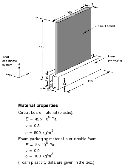
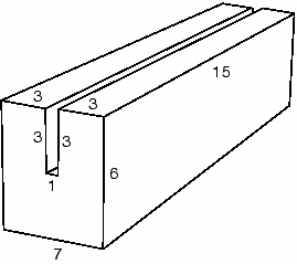
In this example you will investigate the behavior of a circuit board in protective crushable foam packaging dropped at an angle onto a rigid surface. Your goal is to assess whether the foam packaging is adequate to prevent circuit board damage when the board is dropped from a height of 1 meter. You will use the general contact capability in Abaqus/Explicit to model the interactions between the different components. Figure 12–65 shows the dimensions of the circuit board and foam packaging in millimeters and the material properties.
Create the model for this simulation with Abaqus/CAE. Abaqus provides scripts that replicate the complete analysis model for this problem. Run one of these scripts if you encounter difficulties following the instructions given below or if you wish to check your work. Scripts are available in the following locations:
A Python script for this example is provided in “Circuit board drop test,” Section A.14. Instructions on how to fetch the script and run it within Abaqus/CAE are given in Appendix A, “Example Files.”
A plug-in script for this example is available in the Abaqus/CAE Plug-in toolset. To run the script from Abaqus/CAE, select Plug-ins![]() Abaqus
Abaqus![]() Getting Started; highlight Circuit board drop test; and click Run. For more information about the Getting Started plug-ins, see “Running the Getting Started with Abaqus examples,” Section 82.1 of the Abaqus/CAE User's Guide.
Getting Started; highlight Circuit board drop test; and click Run. For more information about the Getting Started plug-ins, see “Running the Getting Started with Abaqus examples,” Section 82.1 of the Abaqus/CAE User's Guide.
Defining the model geometry
You will create three parts representing the packaging, the circuit board, and the floor. The chips will be represented using discrete point masses. You will also create a number of datum points to aid in positioning the part instances and the point masses.
To define the packaging geometry:
The packaging is a three-dimensional solid structure. Create a three-dimensional, deformable part with an extruded solid base feature to represent the packaging; name the part Packaging. Use an approximate part size of 0.1, and sketch a 0.02 m × 0.024 m rectangle as the profile. Specify 0.11 m as the extrusion depth.
From the main menu bar, select Shape![]() Cut
Cut![]() Extrude to create the cut in the packaging in which the circuit board will rest.
Extrude to create the cut in the packaging in which the circuit board will rest.
Select the left end of the packaging as the plane for the extruded cut. Select a vertical line on the packaging profile to be vertical and on the right in the sketching plane.
In the Sketcher, use the vertical construction line tool ![]() to create a vertical construction line through the center of the packaging. Apply a fixed constraint to the construction line.
to create a vertical construction line through the center of the packaging. Apply a fixed constraint to the construction line.
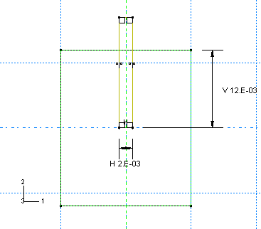
Sketch the profile of the cut shown in Figure 12–66. Use a Symmetry constraint to center the cut about the construction line and edit the dimensions of the cut profile so that it is 0.002 m wide and extends a distance of 0.012 m into the packaging.
In the Edit Cut Extrusion dialog box that appears upon completion of the sketch, select Through All as the end condition and select the arrow direction representing a cut into the packaging.
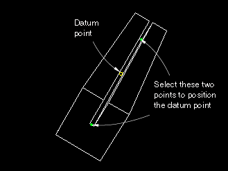
Create a datum point centered on the bottom face of the cut, as shown in Figure 12–67. This point will be used to position the board relative to the packaging.
From the main menu bar, select Tools![]() Datum.
Datum.
The Create Datum dialog box appears.
Accept the default selection of Point as the datum type and select Midway between 2 points as the method.
Select the two points centered on the bottom face at either end of the cut to be the two points between which the datum point will be created.
Abaqus/CAE creates the datum point shown in Figure 12–67.
To define the circuit board geometry:
The circuit board can be modeled as a thin, flat plate with chips attached to it. Create a three-dimensional, deformable planar shell to represent the circuit board; name the part Board. Use an approximate part size of 0.5, and sketch a 0.100 m × 0.150 m rectangle for the profile.
Create the three datum points shown in Figure 12–68. These points will be used to position the chips on the board.
Figure 12–68 Datum points used to position the chips relative to the board. Numbers in parentheses are (x, y) coordinates in meters based on a local origin at the bottom left corner of the circuit board.
From the main menu bar, select Tools![]() Datum.
Datum.
The Create Datum dialog box appears.
Accept the default selection of Point as the datum type, and select Offset from point as the method.
Select the bottom left corner of the board as the point from which to offset, and enter the coordinates for one of the points shown in Figure 12–68.
Repeat Step c to create the other two datum points.
To define the floor:
The surface that the circuit board will impact is effectively rigid. Create a three-dimensional, discrete rigid planar shell to represent the floor; name the part Floor. Use an approximate part size of 0.5. The rigid surface should be large enough to keep any deformable bodies from falling off the edges.
Sketch a 0.2 m × 0.2 m square as the profile. To simplify the positioning of parts in the assembly of the model, ensure that the center of the surface corresponds to point (0, 0) in the sketcher. This also corresponds to the origin of the global coordinate system.
Assign a reference point at the center of the part.
Defining the material and section properties
The circuit board is assumed to be made of a PCB elastic material with a Young's modulus of 45 × 109 Pa and a Poisson's ratio of 0.3. The mass density of the board is 500 kg/m3. Define a material named PCB with these properties.
The foam packaging material will be modeled using the crushable foam plasticity model. The elastic properties of the packaging include a Young's modulus of 3 × 10⁶ Pa and a Poisson's ratio of 0.0. The material density of the packaging is 100 kg/m3. Define a material named Foam with these properties; do not close the material editor.
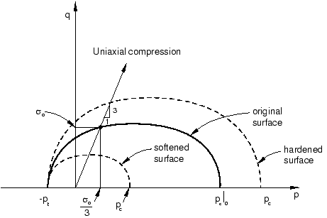
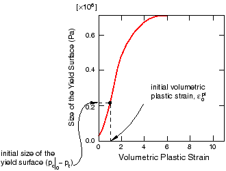
The yield surface of a crushable foam in the p–q (pressure stress-Mises equivalent stress) plane is illustrated in Figure 12–69.
The initial yield behavior is governed by the ratio of initial yield stress in uniaxial compression to initial yield stress in hydrostatic compression,Hardening effects are also included in the material model definition. Table 12–4 summarizes the yield stress–plastic strain data.
Table 12–4 Yield stress–plastic strain data for the crushable foam model.
| Yield stress in uniaxial compression (Pa) | Plastic strain |
|---|---|
| 0.22000E6 | 0.0 |
| 0.24651E6 | 0.1 |
| 0.27294E6 | 0.2 |
| 0.29902E6 | 0.3 |
| 0.32455E6 | 0.4 |
| 0.34935E6 | 0.5 |
| 0.37326E6 | 0.6 |
| 0.39617E6 | 0.7 |
| 0.41801E6 | 0.8 |
| 0.43872E6 | 0.9 |
| 0.45827E6 | 1.0 |
| 0.49384E6 | 1.2 |
| 0.52484E6 | 1.4 |
| 0.55153E6 | 1.6 |
| 0.57431E6 | 1.8 |
| 0.59359E6 | 2.0 |
| 0.62936E6 | 2.5 |
| 0.65199E6 | 3.0 |
| 0.68334E6 | 5.0 |
| 0.68833E6 | 10.0 |
abaqus fetch job=drop*.txtIn the material editor, select Mechanical
Define a homogeneous shell section named BoardSection that refers to the material PCB. Specify a thickness of 0.002 m, and assign this section definition to the part Board. Define a homogeneous solid section named FoamSection that refers to the material Foam. Assign this section definition to the part Packaging.
For the circuit board it is most meaningful to output stress results in the longitudinal and lateral directions, aligned with the edges of the board. Therefore, you need to specify a local material orientation for the circuit board mesh.
To specify a material orientation for the board:
Double-click Board underneath the Parts container in the Model Tree.
To define a datum coordinate system for the orientation:
From the main menu bar, select Tools![]() Datum.
Datum.
Select CSYS as the type and 2 lines as the method.
In the Create Datum CSYS dialog box that appears, select a rectangular coordinate system and click Continue.
In the viewport, select the bottom horizontal edge of the board to be the local x-axis and the right vertical edge of the board to lie in the X–Y plane.
The datum coordinate system appears in yellow in the viewport.
From the main menu bar of the Property module, select Assign![]() Material Orientation. In the viewport select the circuit board. Select the datum coordinate system as the coordinate system. In the material orientation editor select Axis 3 as the shell surface normal and None as the additional rotation about that axis.
Material Orientation. In the viewport select the circuit board. Select the datum coordinate system as the coordinate system. In the material orientation editor select Axis 3 as the shell surface normal and None as the additional rotation about that axis.
The material orientation appears on the board in the viewport.
Creating the assembly
In the Model Tree, double-click Instances underneath the Assembly container and create a dependent instance of the floor.
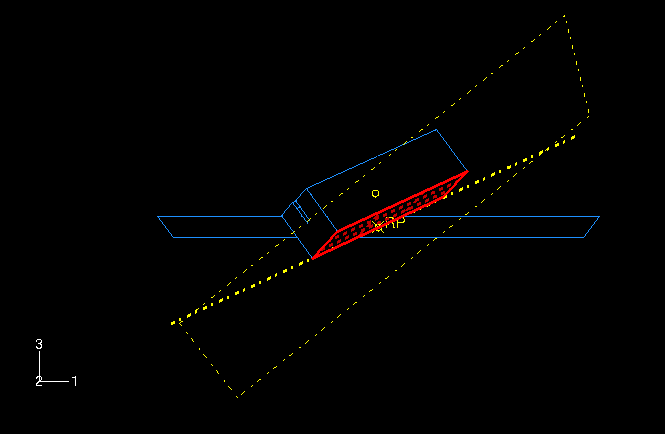
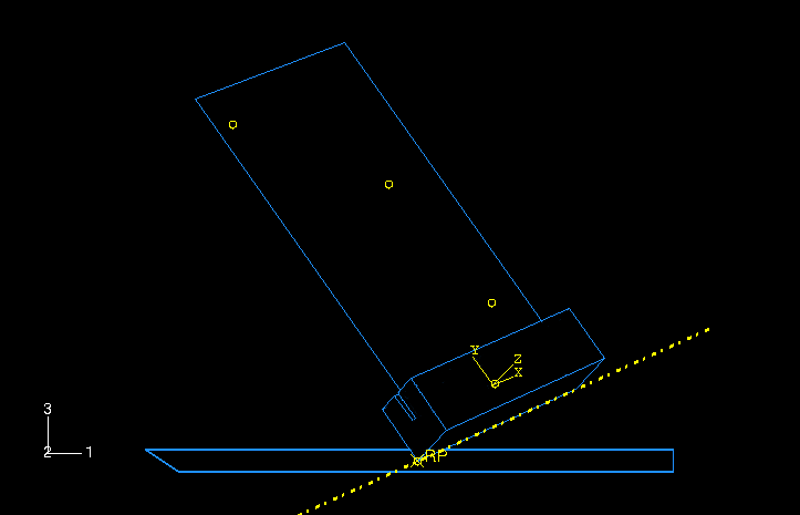
The circuit board will be dropped at an angle; the final model assembly is shown in Figure 12–71.
You will use the positioning tools in the Assembly module to position the packaging first; then you will position the board relative to the packaging. Finally, you will create a reference point at each datum point location of the board to represent the chips.To position the packaging:
From the main menu bar of the Assembly module, select Tools![]() Datum to create additional datum points that will help you position the packaging.
Datum to create additional datum points that will help you position the packaging.
Select Point as the type, and select Enter coordinates as the method.
Create two datum points at (0, 0, 0) and (0.5, 0.707, 0.25).
Click the auto-fit tool to see both points in the viewport.
In the Create Datum dialog box, select Axis as the type and 2 points as the method. Create a datum axis defined by the two datum points created in the previous step, selecting the point at (0.5, 0.707, 0.25) as the first point in the datum axis definition.
Tip: Use the Selection toolbar to restrict your selection to Datums.
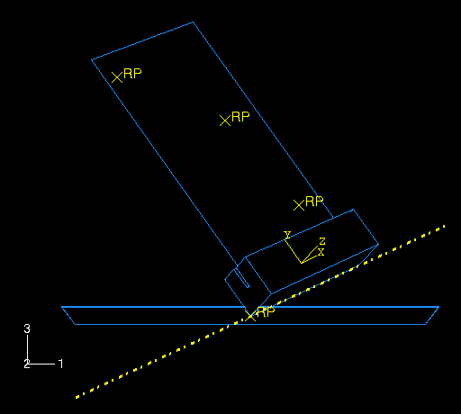
Instance the packaging.
Constrain the packaging so that the bottom edge aligns with the datum axis.
From the main menu bar, select Constraint![]() Edge to Edge.
Edge to Edge.
Select the edge of the packaging shown in Figure 12–72 as a straight edge of the movable instance.
Tip:
To obtain a better view of the model, select View![]() Specify from the main menu bar and select Viewpoint as the method; enter (1, 1, 1) for the viewpoint vector and (0, 0, 1) for the up vector.
Specify from the main menu bar and select Viewpoint as the method; enter (1, 1, 1) for the viewpoint vector and (0, 0, 1) for the up vector.
Select the datum axis as the fixed instance.
If necessary, click Flip in the prompt area to reverse the direction of the arrow on the packaging; click OK when the arrows point in opposite directions as shown in Figure 12–72.
Tip: You may need to zoom out and rotate the model to see the arrow on the datum axis. The direction of this arrow depends on how you defined the axis initially; if the arrow on your axis points in the reverse direction of the one shown in the figure, the arrow on your packaging should also be opposite to the figure.
Abaqus/CAE positions the packaging as shown in Figure 12–73.
Note: Abaqus/CAE stores position constraints as features of the assembly; if you make a mistake while positioning the assembly, you can delete the position constraints. Simply click mouse button 3 on the constraint you wish to delete in the list of Position Constraints items found underneath the Assembly container in the Model Tree, and select Delete from the menu that appears.
Create a third datum point at (0.5, 0.707, 0.5), and click the auto-fit tool again.
In the Create Datum dialog box, select Plane as the type and Line and point as the method. Create a datum plane defined by the datum axis created earlier and the datum point created in the previous step.
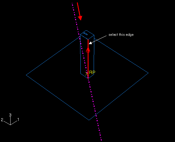
Constrain the packaging so that the bottom face lies on the datum plane.
From the main menu bar, select Constraint![]() Face to Face.
Face to Face.
Select the face of the packaging shown in Figure 12–74 as a face of the movable instance.
Select the datum plane as the fixed instance.
If necessary, click Flip in the prompt area; click OK when both arrows point in the same direction.
Accept the default distance of 0.0 from the fixed plane.
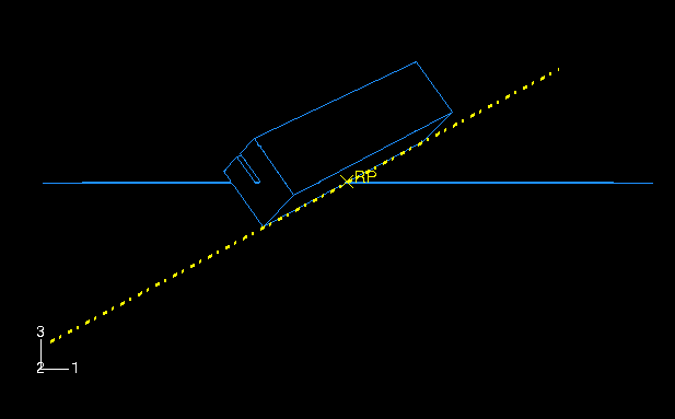
Finally, constrain the packaging to contact the floor at its center.
From the main menu bar, select Constraint![]() Coincident Point.
Coincident Point.
Select the lowest vertex of the packaging as a point on the movable instance, and select the reference point on the floor as a point on the fixed instance.
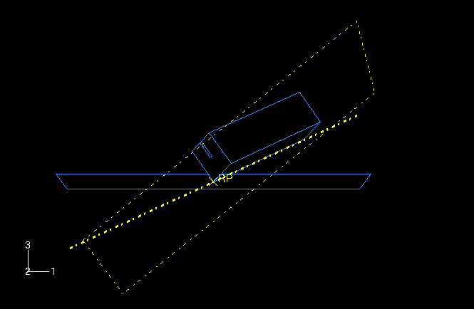
Abaqus/CAE positions the packaging as shown in Figure 12–75.
Now, translate the floor slightly downward to ensure that there is no initial overclosure between the packaging and the floor.
Convert the relative position constraints to absolute constraints to avoid conflicts. From the main menu bar, select Instance![]() Convert Constraints. Select the packaging in the viewport, and click Done in the prompt area.
Convert Constraints. Select the packaging in the viewport, and click Done in the prompt area.
From the main menu bar, select Instance![]() Translate.
Translate.
Select the floor in the viewport.
Enter (0.0, 0.0, 0.0) as the start point for the translation vector and (0.0, 0.0, 0.0001) as the end point for the translation vector.
Click OK to accept the new position.
To position the circuit board:
Instance the circuit board. In the Create Instance dialog box, toggle on Auto-offset from other instances.
From the main menu bar, select Constraint![]() Parallel Face. Select the face of the board as a face on the movable instance; select a face on the long side of the packaging as a face on the fixed instance. If necessary, click Flip in the prompt area to ensure that the arrows on both faces point in the directions shown in Figure 12–76; click OK to complete the constraint.
Parallel Face. Select the face of the board as a face on the movable instance; select a face on the long side of the packaging as a face on the fixed instance. If necessary, click Flip in the prompt area to ensure that the arrows on both faces point in the directions shown in Figure 12–76; click OK to complete the constraint.
From the main menu bar, select Constraint![]() Parallel Edge. Select the top edge of the board as an edge on the movable instance. Select an edge along the length of the packaging as an edge on the fixed instance. If necessary, click Flip in the prompt area to ensure that the arrows on both edges point in the same direction, as shown in Figure 12–77; click OK to complete the constraint.
Parallel Edge. Select the top edge of the board as an edge on the movable instance. Select an edge along the length of the packaging as an edge on the fixed instance. If necessary, click Flip in the prompt area to ensure that the arrows on both edges point in the same direction, as shown in Figure 12–77; click OK to complete the constraint.
From the main menu bar, select Constraint![]() Coincident Point. Select the midpoint of the bottom of the board as a point on the movable instance. Select the datum point at the center of the cut in the packaging as a point on the fixed instance.
Coincident Point. Select the midpoint of the bottom of the board as a point on the movable instance. Select the datum point at the center of the cut in the packaging as a point on the fixed instance.
Tip: Use the Selection toolbar to restrict your selection to Datums.
Figure 12–78 shows the final position of the circuit board. The circuit board and the slot in the packaging are the same thickness (2 mm) so there is a snug fit between the two bodies.
To create the chips:
Create a reference point at each of the three datum point locations on the board to represent each chip. Each of these reference points will later be assigned mass properties. To create a reference point, select Tools![]() Reference Point from the main menu bar of the Assembly module.
Reference Point from the main menu bar of the Assembly module.
Once you have created the reference points, the assembly is complete.
TopChip for the reference point of the top chip
MidChip for the reference point of the middle chip
BotChip for the reference point of the bottom chip
BotBoard for the bottom edge of the board
Defining the step and requesting output
Create a single dynamic, explicit step named Drop; set the time period to 0.02 s. Accept the default history and field output requests. In addition, request vertical displacement (U3), velocity (V3), and acceleration (A3) history output every 7 × 10⁵ s for each of the three chips.
Tip: Define the history output request for the first chip; using the History Output Requests Manager, copy the request and edit the domain to define the requests for the other chips.
Defining contact
Either contact algorithm in Abaqus/Explicit could be used for this problem. However, the definition of contact using the contact pair algorithm would be more cumbersome since, unlike general contact, the surfaces involved in contact pairs cannot span more than one body. We use the general contact algorithm in this example to demonstrate the simplicity of the contact definition for more complex geometries.
Define a contact interaction property named Fric. In the Edit Contact Property dialog box, select Mechanical![]() Tangential Behavior, select Penalty as the friction formulation, and specify a friction coefficient of 0.3 in the table. Accept all other defaults.
Tangential Behavior, select Penalty as the friction formulation, and specify a friction coefficient of 0.3 in the table. Accept all other defaults.
Create a General contact (Explicit) interaction named All in the Drop step. In the Edit Interaction dialog box, accept the default selection of All* with self for the Contact Domain to specify self-contact for the default unnamed, all-inclusive surface defined automatically by Abaqus/Explicit. This method is the simplest way to define contact in Abaqus/Explicit for an entire model. Select Fric as the Global property assignment, and click OK.
Defining tie constraints
You will use tie constraints to attach the chips to the board. Begin by defining a surface named Board for the circuit board. Select Both sides in the prompt area to specify that the surface is double-sided. In the Model Tree, double-click the Constraints container; define a tie constraint named TopChip. Select Board as the master surface and TopChip as the slave node region. Toggle off Tie rotational DOFs if applicable in the Edit Constraint dialog box since only the effects of the chip masses are of interest, and click OK. Yellow circles appear on the model to represent the constraint. Similarly, create tie constraints named MidChip and BotChip for the middle and bottom chips.
Assigning mass properties to the chips:
You will assign a point mass to each chip. To do this, expand Engineering Features underneath the Assembly container in the Model Tree. In the list that appears, double-click Inertias. In the Create Inertia dialog box, enter the name MassTopChip and click Continue. Select the set TopChip, and assign it a mass of 0.005 kg. Repeat this procedure for the two remaining chips.
Specifying loads and boundary conditions
Constrain the reference point on the floor in all directions; for example, you could prescribe an ENCASTRE boundary condition.
Two methods could be used to simulate the circuit board being dropped from a height of 1 m. You could model the circuit board and foam at a height of 1 m above the floor and allow Abaqus/Explicit to calculate the motion under the influence of gravity; however, this method is impractical because of the large number of increments required to complete the “free-fall” part of the simulation. The more efficient method is to model the circuit board and packaging in an initial position very close to the surface of the floor (as you have done in this problem) and specify an initial velocity of 4.43 m/s to simulate the 1 m drop. Create a predefined field in the initial step to specify an initial velocity of V3 = 4.43 m/s for the board, chips, and packaging.
Meshing the model and defining a job
Seed the circuit board with 10 elements along its length and height. Seed the edges of the packaging as shown in Figure 12–79.
The mesh for the packaging will be too coarse near the impacting corner to provide highly accurate results; however, it will be adequate for a low-cost preliminary study. Using the swept mesh technique (with the medial axis algorithm), mesh the packaging with C3D8R elements and the board with S4R elements from the Abaqus/Explicit library. Use enhanced hourglass control for the packaging mesh to control hourglassing effects. Specify a global seed of 1.0 for the floor, and mesh it with one Abaqus/Explicit R3D4 element.Note: The suggested mesh density exceeds the model size limits of the Abaqus Student Edition. Specify 12 elements along the length of the foam packaging if using this product.
Create a job named Circuit, and give it the following description: Circuit board drop test. Double precision should be used for this analysis to minimize the noise in the solution. In the Precision tabbed page of the job editor, select Double-analysis only as the Abaqus/Explicit precision. Save your model to a model database file, and submit the job for analysis. Monitor the solution progress; correct any modeling errors that are detected, and investigate the cause of any warning messages.
Enter the Visualization module, and open the output database file created by this job (Circuit.odb).
Checking material directions
The material directions obtained from the orientation definition can be checked in the Visualization module.
To plot the material orientation:
First, change the view to a more convenient setting. If it is not visible, display the Views toolbar by selecting View![]() Toolbars
Toolbars![]() Views from the main menu bar. In the Views toolbar, select the X–Z setting.
Views from the main menu bar. In the Views toolbar, select the X–Z setting.
From the main menu bar, select Plot![]() Material Orientations
Material Orientations![]() On Deformed Shape.
On Deformed Shape.
The orientations of the material directions for the circuit board at the end of the simulation are shown. The material directions are drawn in different colors. The material 1-direction is blue, the material 2-direction is yellow, and the 3-direction, if it is present, is red.
To view the initial material orientation, select Result![]() Step/Frame. In the Step/Frame dialog box that appears, select Increment 0. Click Apply.
Step/Frame. In the Step/Frame dialog box that appears, select Increment 0. Click Apply.
Abaqus displays the initial material directions.
To restore the display to the results at the end of the analysis, select the last increment available in the Step/Frame dialog box; and click OK.
Animation of results
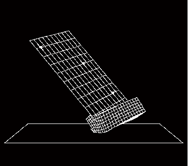
You will create a time-history animation of the deformation to help you visualize the motion and deformation of the circuit board and foam packaging during impact.
To create a time-history animation:
Plot the deformed model shape at the end of the analysis.
From the main menu bar, select Animate![]() Time History.
Time History.
The animation of the deformed model shape begins.
From the main menu bar, select View![]() Parallel to turn off perspective.
Parallel to turn off perspective.
In the context bar, click ![]() to pause the animation after a full cycle has been completed.
to pause the animation after a full cycle has been completed.
In the context bar, click ![]() and then select a node on the foam packaging near one of the corners that impacts the floor. When you restart the animation the camera will move with the selected node. If you zoom in on the node, it will remain in view throughout the animation.
and then select a node on the foam packaging near one of the corners that impacts the floor. When you restart the animation the camera will move with the selected node. If you zoom in on the node, it will remain in view throughout the animation.
Note:
To reset the camera to follow the global coordinate system, click ![]() in the context bar.
in the context bar.
Plotting model energy histories
Plot graphs of various energy variables versus time. Energy output can help you evaluate whether an Abaqus/Explicit simulation is predicting an appropriate response.
To plot energy histories:
In the Results Tree, click mouse button 3 on History Output for the output database named Circuit.odb. From the menu that appears, select Filter.
In the filter field, enter *ALL* to restrict the history output to just the energy output variables.
Select the ALLAE output variable, and save the data as Artificial Energy.
Select the ALLIE output variable, and save the data as Internal Energy.
Select the ALLKE output variable, and save the data as Kinetic Energy.
Select the ALLPD output variable, and save the data as Plastic Dissipation.
Select the ALLSE output variable, and save the data as Strain Energy.
In the Results Tree, expand the XYData container.
Select all five curves. Click mouse button 3, and select Plot from the menu that appears to view the X–Y plot.
Next, you will customize the appearance of the plot; begin by changing the line styles of the curves.
Open the Curve Options dialog box.
In this dialog box, apply different line styles and thicknesses to each of the curves displayed in the viewport.
Next, reposition the legend so that it appears inside the plot.
Double-click the legend to open the Chart Legend Options dialog box.
In this dialog box, switch to the Area tabbed page, and toggle on Inset.
In the viewport, drag the legend over the plot.
Now change the format of the X-axis labels.
In the viewport, double-click the X-axis to access the X Axis options in the Axis Options dialog box.
In this dialog box, switch to the Axes tabbed page, and select the Engineering label format for the X-axis.
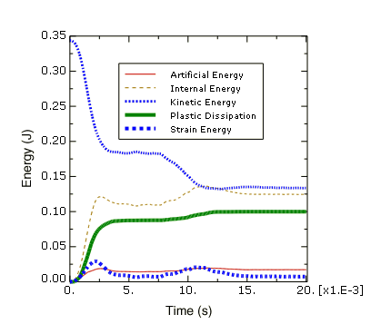
The energy histories appear as shown in Figure 12–81.
First, consider the kinetic energy history. At the beginning of the simulation the components are in free fall, and the kinetic energy is large. The initial impact deforms the foam packaging, thus reducing the kinetic energy. The components then bounce and rotate about the impacted corner until the opposite side of the foam packaging impacts the floor at about 8 ms, further reducing the kinetic energy.
The deformation of the foam packaging during impact causes a transfer of kinetic energy to internal energy in the foam packaging and the circuit board. From Figure 12–81 we can see that the internal energy increases as the kinetic energy decreases. In fact, the internal energy is composed of elastic energy and plastically dissipated energy, both of which are also plotted in Figure 12–81. Elastic energy rises to a peak and then falls as the elastic deformation recovers, but the plastically dissipated energy continues to rise as the foam is deformed permanently.
Another important energy output variable is the artificial energy, which is a substantial fraction (approximately 15%) of the internal energy in this analysis. By now you should know that the quality of the solution would improve if the artificial energy could be decreased to a smaller fraction of the total internal energy.
What causes high artificial strain energy in this problem?
Contact at a single node—such as the corner impact in this example—can cause hourglassing, especially in a coarse mesh. Two common strategies for reducing the artificial strain energy are to refine the mesh or to round the impacting corner. For the current exercise, however, we shall continue with the original mesh, realizing that improving the mesh would lead to an improved solution.
Evaluating acceleration histories at the chips
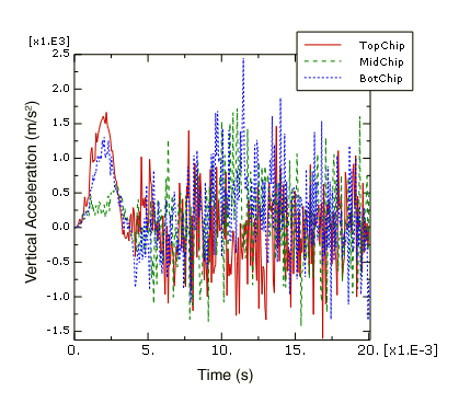
The next result we wish to examine is the acceleration of the chips attached to the circuit board. Excessive accelerations during impact may damage the chips. Therefore, in order to assess the desirability of the foam packaging, we need to plot the acceleration histories of the three chips. Since we expect the accelerations to be greatest in the 3-direction, we will plot the variable A3.
To plot acceleration histories:
In the Results Tree, filter the History Output container according to *A3*; select the acceleration A3 of the nodes in sets TopChip, MidChip, and BotChip; and plot the three X–Y data objects.
The X–Y plot appears in the viewport. As before, customize the plot appearance to obtain a plot similar to Figure 12–82.
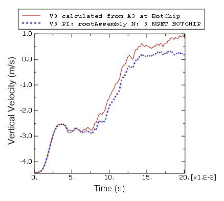
Next, we will evaluate the plausibility of the acceleration data recorded at the bottom chip. To do this, we will integrate the acceleration data to calculate the chip velocity and displacement and compare the results to the velocity and displacement data recorded directly by Abaqus/Explicit.
To integrate the bottom chip acceleration history:
In the Results Tree, filter the History Output container according to *BOTCHIP*, select the acceleration A3 of the node in set BotChip, and save the data as A3.
In the Results Tree, double-click XYData; then select Operate on XY data in the Create XY Data dialog box. Click Continue.
In the Operate on XY Data dialog box, integrate acceleration A3 to calculate velocity and subtract the initial velocity magnitude of 4.43 m/s. The expression at the top of the dialog box should appear as:
integrate ( "A3" ) - 4.43
Click Plot Expression to plot the calculated velocity curve.
In the Results Tree, click mouse button 3 on the velocity V3 history output for the node in set BotChip; and select Add to Plot from the menu that appears.
The X–Y plot appears in the viewport. As before, customize the plot appearance to obtain a plot similar to Figure 12–83. The velocity curve you produced by integrating the acceleration data may be different from the one pictured here. The reason for this will be discussed later.
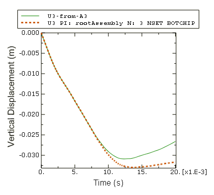
In the Operate on XY Data dialog box, integrate acceleration A3 a second time to calculate chip displacement. The expression at the top of the dialog box should appear as:
integrate ( integrate ( "A3" ) - 4.43 )
Click Plot Expression to plot the calculated displacement curve.
Notice that the Y-value type is length. In order to plot the calculated displacement with the same Y-axis as the displacement output recorded during the analysis, we must save the X–Y data and change the Y-value type to displacement.
Click Save As to save the calculated displacement curve as U3-from-A3.
In the XYData container of the Results Tree, click mouse button 3 on U3-from-A3; and select Edit from the menu that appears.
In the Edit XY Data dialog box, choose Displacement as the Y-value type.
In the Results Tree, double-click U3–from-A3 to recreate the calculated displacement plot with the displacement Y-value type.
In the Results Tree, click mouse button 3 on the displacement U3 history output for the node in set BotChip; and select Add to Plot from the menu that appears.
The X–Y plot appears in the viewport. As before, customize the plot appearance to obtain a plot similar to Figure 12–84. Again, the curve you produced by integrating the acceleration data may be different from the one pictured here. The reason for this will be discussed later.
Why are the velocity and displacement curves calculated by integrating the acceleration data different from the velocity and displacement recorded during the analysis?
In this example the acceleration data has been corrupted by a phenomenon called aliasing. Aliasing is a form of data corruption that occurs when a signal (such as the results of an Abaqus analysis) is sampled at a series of discrete points in time, but not enough data points are saved in order to correctly describe the signal. The aliasing phenomenon can be addressed using digital signal processing (DSP) methods, a fundamental principle of which is the Nyquist Sampling Theorem (also known as the Shannon Sampling Theorem). The Sampling Theorem requires that a signal be sampled at a rate that is greater than twice the signal's highest frequency. Therefore, the maximum frequency content that can be described by a given sampling rate is half that rate (the Nyquist frequency). Sampling (storing) a signal with large-amplitude oscillations at frequencies greater than the Nyquist frequency of the sample rate may produce significantly distorted results due to aliasing. In this example the chip acceleration was sampled every 0.07 ms, which is a sampling rate of 14.3 kHz (the sample rate is the inverse of the sample size). The recorded data was aliased because the chip acceleration response has frequency content above 7.2 kHz (half the sample rate).
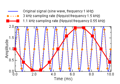
Aliasing of a sine wave
To better understand how aliasing distorts data, consider a 1 kHz sine wave sampled using various sampling rates, as shown in Figure 12–85.
According to the Sampling Theorem, this signal must be sampled at a rate greater than 2 kHz to avoid alias distortions. We will evaluate what happens when the sample rate is greater than or less than this value.Consider the data recorded with a sample rate of 1.1 kHz; this rate is less than the required 2 kHz rate. The resulting curve exhibits alias distortions because it is an extremely misleading representation of the original 1 kHz sine wave.
Now consider the data recorded with a sample rate of 3 kHz; this rate is greater than the required 2 kHz rate. The frequency content of the original signal is captured without aliasing. However, this sample rate is not high enough to guarantee that the peak values of the sampled signal are captured very accurately. To guarantee 95% accuracy of the recorded local peak values, the sampling rate must exceed the signal frequency by a factor of ten or more.
Avoiding aliasing
In the previous two examples of aliasing (the aliased chip acceleration and the aliased sine wave), it would not have been obvious from the aliased data alone that aliasing had occurred. In addition, there is no way to uniquely reconstruct the original signal from the aliased data alone. Therefore, care should be taken to avoid aliasing your analysis results, particularly in situations when aliasing is most likely to occur.
Susceptibility to aliasing depends on a number of factors, including output rate, output variable, and model characteristics. Recall that signals with large-amplitude oscillations at frequencies greater than half the sampling rate (the Nyquist frequency) may be significantly distorted due to aliasing. The two output variables that are most likely to have large-amplitude high-frequency content are accelerations and reaction forces. Therefore, these variables are the most susceptible to aliasing. Displacements, on the other hand, are lower in frequency content by nature, so they are much less susceptible to aliasing. Other result variables, such as stress and strain, fall somewhere in between these two extremes. Any model characteristic that reduces the high-frequency response of the solution will decrease the analysis’s susceptibility to aliasing. For example, an elastically dominated impact problem would be even more susceptible to aliasing than this circuit board drop test which includes energy absorbing packaging.
The safest way to ensure that aliasing is not a problem in your results is to request output at every increment. When you do this, the output rate is determined by the stable time increment, which is based on the highest possible frequency response of the model. However, requesting output at every increment is often not practical because it would result in very large output files. In addition, output at every increment is usually much more data than you need; there is no need to capture high-frequency solution noise when what you are really interested in is the lower-frequency structural response. An alternative method for avoiding aliasing is to request output at a lower rate and use the Abaqus/Explicit real-time filtering capabilities to remove high-frequency content from the result before writing data to the output database file. This technique uses less disk space than requesting output every increment; however, it is up to you to ensure that your output rate and filter choices are appropriate (to avoid aliasing or other distortions related to digital signal processing).
Abaqus/Explicit offers filtering capabilities for both field and history data. Filtering of history data only is discussed here.
In this section you will add real-time filters to the history output requests for the circuit board drop test analysis. While Abaqus/Explicit does allow you to create user-defined output filters (Butterworth, Chebyshev Type I, and Chebyshev Type II) based on criteria that you specify, in this example we will use the built-in antialiasing filter. The built-in antialiasing filter is designed to give you the best un-aliased representation of the results recorded at the output rate you specify on the output request. To do this, Abaqus/Explicit internally applies a low-pass, second-order, Butterworth filter with a cutoff frequency set to one-sixth of the sampling rate. For more information, see “Overview of filtering Abaqus history output” in the Dassault Systèmes Knowledge Base at www.3ds.com/support/knowledge-base. For more information on defining your own real-time filters, see “Filtering output and operating on output in Abaqus/Explicit” in “Output to the output database,” Section 4.1.3 of the Abaqus Analysis User's Guide.
Modifying the history output requests
When Abaqus writes nodal history output to the output database, it gives each data object a name that indicates the recorded output variable, the filter used (if any), the part instance name, the node number, and the node set. For this exercise you will be creating multiple output requests for the node in set BotChip that differ only by the output sample rate, which is not a component of the history output name. To easily distinguish between the similar output requests, create two new sets for the bottom chip reference node. Name one of the new sets BotChip-all and the other BotChip-largeInc.
Next, copy the history output request for the bottom chip three times. Edit the first copy to activate the Antialiasing filter; for this request continue to record data every 7 × 10⁵ s using the set BotChip. Edit the second copy to record the data at every time increment; apply this output request to the set BotChip-all. Edit the third copy to record the data at every 7 × 10⁴ s; apply this output request to the set BotChip-largeInc and activate the Antialiasing filter. When you are finished, there will be four history output requests for the bottom chip (the original one and the three added here).
Edit the output request for the strains in the set BotBoard in order to activate the Antialiasing filter.
Although we will not be discussing the results here, you may wish to add the Antialiasing filter to the history output request for the displacement, velocity, and acceleration of the node sets MidChip and TopChip.
Save your model database, and submit the job for analysis.
Evaluating the filtered acceleration of the bottom chip
When the analysis completes, test the plausibility of the acceleration history output for the bottom chip recorded every 0.07 ms using the built-in, antialiasing filter. Do this by saving and then integrating the filtered acceleration data (A3_ANTIALIASING for set BotChip) and comparing the results to recorded velocity and displacement data, just as you did earlier for the unfiltered version of these results. This time you should find that the velocity and displacement curves calculated by integrating the filtered acceleration are very similar to the velocity and displacement values written to the output database during the analysis. You may also have noticed that the velocity and displacement results are the same regardless of whether or not the built-in antialiasing filter is used. This is because the highest frequency content of the nodal velocity and displacement curves is much less than half the sampling rate. Consequently, no aliasing occurred when the data was recorded without filtering, and when the built-in antialiasing filter was applied it had no effect because there was no high frequency response to remove.
Next, compare the acceleration A3 history output recorded every increment with the two acceleration A3 history curves recorded every 0.07 ms. Plot the data recorded at every increment first so that it does not obscure the other results.
To plot the acceleration histories
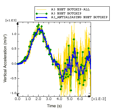
In the Results Tree, filter the History Output container according to *A3*BOTCHIP* and double-click the acceleration A3 history output for the node set BotChip-all.
Select the two acceleration A3 history output objects for the node set BotChip (one filtered with the built-in antialiasing filter and the other with no filtering) using [Ctrl] + Click; click mouse button 3 and select Add to Plot from the menu that appears.
The X–Y plot appears in the viewport. Zoom in to view only the first third of the results and customize the plot appearance to obtain a plot similar to Figure 12–86.
First consider the acceleration history recorded every increment. This curve contains a lot of data, including high-frequency solution noise which becomes so large in magnitude that it obscures the structurally-significant lower-frequency components of the acceleration. When output is requested every increment, the output time increment is the same as the stable time increment, which (in order to ensure stability) is based on a conservative estimate of the highest possible frequency response of the model. Frequencies of structural significance are typically two to four orders of magnitude less than the highest frequency of the model. In this example the stable time increment ranges between 8.4 × 10⁴ ms to 8.8 × 10⁴ ms (see the status file, Circuit.sta), which corresponds to a sample rate of about 1 MHz; this sample rate has been rounded down for this discussion, even though it means that the value is not conservative. Recalling the Sampling Theorem, the highest frequency that can be described by a given sample rate is half that rate; therefore, the highest frequency of this model is about 500 kHz and typical structural frequencies could be as high as 2–3 kHz (more than 2 orders of magnitude less than the highest model frequency). While the output recorded every increment contains a lot of undesirable solution noise in the 3 to 500 kHz range, it is guaranteed to be good (not aliased) data, which can be filtered later with a postprocessing operation if necessary.
Next consider the data recorded every 0.07 ms without any filtering. Recall that this is the curve we know to be corrupted by aliasing. The curve jumps from point to point by directly including whatever the raw acceleration value happens to be after each 0.07 ms interval. The variable nature of the high-frequency noise makes this aliased result very sensitive to otherwise imperceptible variations in the solution (due to differences between computer platforms, for example), hence the results you recorded every 0.07 increments may be significantly different from those shown in Figure 12–86. Similarly, the velocity and displacement curves we produced by integrating the aliased acceleration (Figure 12–83 and Figure 12–84) data are extremely sensitive to small differences in the solution noise.
When the built-in antialiasing filter is applied to the output requested every 0.07 ms, frequency content that is too high to be captured by the 14.3 kHz sample rate is filtered out before the result is written to the output database. To do this, Abaqus internally defines a low-pass, second-order, Butterworth filter. Low-pass filters attenuate the frequency content of a signal that is above a specified cutoff frequency. An ideal low-pass filter would completely eliminate all frequencies above the cutoff frequency while having no effect on the frequency content below the cutoff frequency. In reality there is a transition band of frequencies surrounding the cutoff frequency that are partially attenuated. To compensate for this, the built-in antialiasing filter has a cutoff frequency that is one-sixth of the sample rate, a value lower than the Nyquist frequency of one-half the sample rate. In most cases (including this example), this cutoff frequency is adequate to ensure that all frequency content above the Nyquist frequency has been removed before the data are written to the output database.
Abaqus/Explicit does not check to ensure that the specified output time interval provides an appropriate cutoff frequency for the internal antialiasing filter; for example, Abaqus does not check that only the noise of the signal is eliminated. When the acceleration data are recorded every 0.07 ms, the internal antialiasing filter is applied with a cutoff frequency of 2.4 kHz. This cutoff frequency is nearly the same value we previously determined to be the maximum physically meaningful frequency for the model (more than two orders of magnitude less than the maximum frequency the stable time increment can capture). The 0.07 ms output interval was intentionally chosen for this example to avoid filtering frequency content that could be physically meaningful. Next, we will study the results when the antialiasing filter is applied with a sample interval that is too large.
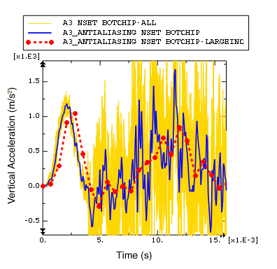
To plot the filtered acceleration histories
In the Results Tree, double-click the acceleration A3 history output for the node set BotChip-all.
Select the two filtered acceleration A3_ANTIALIASING history output objects for the bottom chip; click mouse button 3 and select Add to Plot from the menu that appears.
The X–Y plot appears in the viewport. Zoom out and customize the plot appearance to obtain a plot similar to Figure 12–87.
Figure 12–87 clearly illustrates some of the problems that can arise when the built-in antialiasing filter is used with too large an output time increment. First, notice that many of the oscillations in the acceleration output are filtered out when the acceleration is recorded with large time increments. In this dynamic impact problem it is likely that a significant portion of the removed frequency content is physically meaningful. Previously, we estimated that the frequency of the structural response may be as large as 2–3 kHz; however, when the sample interval is 0.7 ms, filtering is performed with a low cutoff frequency of 0.24 kHz (sample interval of 0.7 ms corresponds to a sample frequency of 1.43 kHz, one-sixth of which is the 0.24 kHz cutoff frequency). Even though the results recorded every 0.7 ms may not capture all physically meaningful frequency content, it does capture the low-frequency content of the acceleration data without distortions due to aliasing. Keep in mind that filtering decreases the peak value estimations, which is desirable if only solution noise is filtered, but can be misleading when physically meaningful solution variations have been removed.
Another issue to note is that there is a time delay in the acceleration results recorded every 0.7 ms. This time delay (or phase shift) affects all real-time filters. The filter must have some input in order to produce output; consequently the filtered result will include some time delay. While some time delay is introduced for all real-time filtering, the time delay becomes more pronounced as the filter cutoff frequency decreases; the filter must have input over a longer span of time in order to remove lower frequency content. Increasing the filter order (an option if you have created a user-defined filter, rather than using the second-order built-in antialiasing filter) also results in an increase in the output time delay. For more information, see “Filtering output and operating on output in Abaqus/Explicit” in “Output to the output database,” Section 4.1.3 of the Abaqus Analysis User's Guide.
Use the real-time filtering functionality with caution. In this example we would not have been able to identify the problems with the heavily filtered data if we did not have appropriate data for comparison. In general it is best to use a minimal amount of filtering in Abaqus/Explicit, so that the output database contains a rich, un-aliased, representation for the solution recorded at a reasonable number of time points (rather than at every increment). If additional filtering is necessary, it can be done as a postprocessing operation in Abaqus/CAE.
Filtering acceleration history in Abaqus/CAE
In this section we will use the Visualization module in Abaqus/CAE to filter the acceleration history data written to the output database. Filtering as a postprocessing operation in the Visualization module has several advantages over the real-time filtering available in Abaqus/Explicit. In the Visualization module you can quickly filter X–Y data and plot the results. You can easily compare the filtered results to the unfiltered results to verify that the filter produced the desired effect. Using this technique you can quickly iterate to find appropriate filter parameters. In addition, the Visualization module filters do not suffer from the time delay that is unavoidable when filtering is applied during the analysis. Keep in mind, however, that postprocessing filters cannot compensate for poor analysis history output; if the data has been aliased or if physically meaningful frequencies have been removed, no postprocessing operation can recover the lost content.
To demonstrate the differences between filtering in the Visualization module and filtering in Abaqus/Explicit, we will filter the acceleration of the bottom chip in the Visualization module and compare the results to the filtered data Abaqus/Explicit wrote to the output database.
To filter acceleration history:
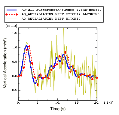
In the Results Tree, select the acceleration A3 history output for the node set BotChip-all, and save the data as A3-all.
In the Results Tree, double-click XYData; then select Operate on XY data in the Create XY Data dialog box. Click Continue.
In the Operate on XY Data dialog box, filter A3-all with filter options that are equivalent to those applied by the Abaqus/Explicit built-in antialiasing filter when the output increment is 0.7 ms. Recall that the built-in antialiasing filter is a second-order Butterworth filter with a cutoff frequency that is one-sixth of the output sample rate; hence, the expression at the top of the dialog box should appear as
butterworthFilter ( xyData="A3-all",
 cutoffFrequency=1/(6*0.0007) )
Click Plot Expression to plot the filtered acceleration curve.
In the Results Tree, click mouse button 3 on the filtered acceleration A3_ANTIALIASING history output for node set BotChip-largeInc; and select Add to Plot from the menu that appears. If you wish, also add the filtered acceleration history for the node set BotChip.
The X–Y plot appears in the viewport. As before, customize the plot appearance to obtain a plot similar to Figure 12–88.
In Figure 12–88 it is clear that the postprocessing filter in the Visualization module of Abaqus/CAE does not suffer from the time delay that occurs when filtering is performed while the analysis is running. This is because the Visualization module filters are bidirectional, which means that the filtering is applied first in a forward pass (which introduces some time delay) and then in a backward pass (which removes the time delay). As a consequence of the bidirectional filtering in the Visualization module, the filtering is essentially applied twice, which results in additional attenuation of the filtered signal compared to the attenuation achieved with a single-pass filter. This is why the local peaks in the acceleration curve filtered in the Visualization module are a bit lower than those in the curve filtered by Abaqus/Explicit.
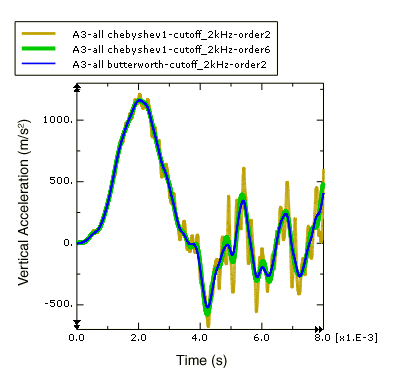
To develop a better understanding of the Visualization module filtering capabilities, return to the Operate on XY Data dialog box and filter the acceleration data with other filter options. For example, try different cutoff frequencies.
Can you confirm that the cutoff frequency of 2.4 kHz associated with the built-in antialiasing filter with a time increment size of 0.07 was appropriate? Does increasing the cutoff frequency to 6 kHz, 7 kHz, or even 10 kHz produce significantly different results?
You should find that a moderate increase in the cutoff frequency does not have a significant effect on the results, implying that we probably have not missed physically meaningful frequency content when we filtered with a cutoff frequency of 2.4 kHz.
Compare the results of filtering the acceleration data with Butterworth and Chebyshev Type I filters. The Chebyshev filter requires a ripple factor parameter (rippleFactor), which indicates how much oscillation you will allow in exchange for an improved filter response; see “Filtering output and operating on output in Abaqus/Explicit” in “Output to the output database,” Section 4.1.3 of the Abaqus Analysis User's Guide for more information. For the Chebyshev Type I filter a ripple factor of 0.071 will result in a very flat pass band with a ripple that is only 0.5%.
You may not notice much difference between the filters when the cutoff frequency is 5 kHz, but what about when the cutoff frequency is 2 kHz? What happens when you increase the order of the Chebyshev Type I filter?
Compare your results to those shown in Figure 12–89.
Note: The Abaqus/CAE postprocessing filters are second-order by default. To define a higher order filter you can use the filterOrder parameter with the butterworthFilter and the chebyshev1Filter operators. For example, use the following expression in the Operate on XY Data dialog box to filter A3-all with a sixth-order Chebyshev Type I filter using a cutoff frequency of 2 kHz and a ripple factor of 0.017.
chebyshev1Filter ( xyData="A3-all" , cutoffFrequency=2000,
 rippleFactor= 0.017, filterOrder=6)
The second-order Chebyshev Type I filter with a ripple factor of 0.071 is a relatively weak filter, so some of the frequency content above the 2 kHz cutoff frequency is not filtered out. When the filter order is increased, the filter response is improved so that the results are more like the equivalent Butterworth filter. For more information on the X–Y data filters available in Abaqus/CAE see “Operating on saved X–Y data objects,” Section 47.4 of the Abaqus/CAE User's Guide.
Filtering strain history in Abaqus/CAE
Strain in the circuit board near the location of the chips is another result that may assist us in determining the effectiveness of the foam packaging. If the strain under the chips exceeds a limiting value, the solder securing the chips to the board will fail. We wish to identify the peak strain in any direction. Therefore, the maximum and minimum principal logarithmic strains are of interest. Principal strains are one of a number of Abaqus results that are derived from nonlinear operators; in this case a nonlinear function is used to calculate principal strains from the individual strain components. Some other common results that are derived from nonlinear operators are principal stresses, Mises stress, and equivalent plastic strains. Care must be taken when filtering results that are derived from nonlinear operators, because nonlinear operators (unlike linear ones) can modify the frequency of the original result. Filtering such a result may have undesirable consequences; for example, if you remove a portion of the frequency content that was introduced by the application of the nonlinear operator, the filtered result will be a distorted representation of the derived quantity. In general, you should either avoid filtering quantities derived from nonlinear operators or filter the underlying quantities before calculating the derived quantity using the nonlinear operator.
The strain history output for this analysis was recorded every 0.07 ms using the built-in antialiasing filter. To verify that the antialiasing filter did not distort the principal strain results, we will calculate the principal logarithmic strains using the filtered strain components and compare the result to the filtered principal logarithmic strains.
To calculate the principal logarithmic strains:
To identify the elements in set BotBoard that are closest to the bottom chip (use the ODB display options to display the mass elements), plot the undeformed circuit board with element numbers visible.
In the Results Tree, filter the History Output according to *LE*Element #*, where # is the number of one of the elements in set BotBoard that is close to the bottom chip. Select the logarithmic strain component LE11 on the SPOS surface of the element, and save the data as LE11.
Similarly, save the LE12 and LE22 strain components for the same element as LE12 and LE22, respectively.
In the Results Tree, double-click XYData; then select Operate on XY data in the Create XY Data dialog box. Click Continue.
In the Operate on XY Data dialog box, use the saved logarithmic strain components to calculate the maximum principal logarithmic strain. The expression at the top of the dialog box should appear as:
(("LE11"+"LE22")/2) + sqrt( power(("LE11"-"LE22")/2,2)
 + power("LE12"/2,2) )
Click Save As to save calculated maximum principal logarithmic strain as LEP-Max.
Edit the expression in the Operate on XY Data dialog box to calculate the minimum principal logarithmic strain. The modified expression should appear as:
(("LE11"+"LE22")/2) - sqrt( power(("LE11"-"LE22")/2,2)
 + power("LE12"/2,2) )
Click Save As to save calculated minimum principal logarithmic strain as LEP-Min.
In order to plot the calculated principal logarithmic strains with the same Y-axis as the strains recorded during the analysis, change the Y-value type to strain.
In the XYData container of the Results Tree, click mouse button 3 on LEP-Max; and select Edit from the menu that appears.
In the Edit XY Data dialog box, choose Strain as the Y-value type.
Similarly, edit LEP-Min and select Strain as the Y-value type.
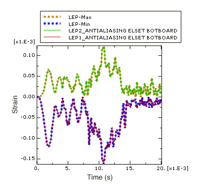
Using the Results Tree, plot LEP-Man and LEP-Min along with the principal strains recorded during the analysis (LEP1 and LEP2) for the same element in set BotBoard.
As before, customize the plot appearance to obtain a plot similar to Figure 12–90. The actual plot will depend on which element you selected.
In Figure 12–90 we see that the filtered principal logarithmic strain curves recorded during the analysis are indistinguishable from the principal logarithmic strain curves calculated from the filtered strain components. Therefore the antialiasing filter (cutoff frequency 2.4 kHz) did not remove any of the frequency content introduced by the nonlinear operation to calculate principal strains form the original strain data. Next, filter the strain data with a lower cutoff frequency of 500 Hz.
To filter principal logarithmic strains with a cutoff frequency of 500 Hz:
In the Results Tree, double-click XYData; then select Operate on XY data in the Create XY Data dialog box. Click Continue.
In the Operate on XY Data dialog box, filter the maximum principal logarithmic strain LEP-Max using a second-order Butterworth filter with a cutoff frequency of 500 Hz. The expression at the top of the dialog box should appear as:
butterworthFilter(xyData="LEP-Max", cutoffFrequency=500)
Click Save As to save the calculated maximum principal logarithmic strain as LEP-Max-FilterAfterCalc-bw500.
Similarly, filter the logarithmic strain components LE11, LE12, and LE22 using the same second-order Butterworth filter with a cutoff frequency of 500 Hz. Save the resulting curves as LE11–bw500, LE12–bw500, and LE22–bw500, respectively.
Now calculate the maximum principal logarithmic strain using the filtered logarithmic strain components. The expression at the top of the Operate on XY Data dialog box should appear as:
(("LE11-bw500"+"LE22-bw500")/2) + sqrt(
 power(("LE11-bw500"-"LE22-bw500")/2,2) +
 power("LE12-bw500"/2,2) )
Click Save As to save the calculated maximum principal logarithmic strain as LEP-Max-CalcAfterFilter-bw500.
In the XYData container of the Results Tree, click mouse button 3 on LEP-Max-CalcAfterFilter-bw500; and select Edit from the menu that appears.
In the Edit XY Data dialog box, choose Strain as the Y-value type.
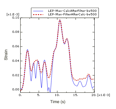
Plot LEP-Max-CalcAfterFilter-bw500 and LEP-Max-FilterAfterCalc-bw500 as shown in Figure 12–91. As before, the actual plot will depend on which element you selected.
In Figure 12–91 you can see that there is a significant difference between filtering the strain data before and after the principal strain calculation. The curve that was filtered after the principal strain calculation is distorted because some of the frequency content introduced by applying the nonlinear principal-stress operator is higher than the 500 Hz filter cutoff frequency. In general, you should avoid directly filtering quantities that have been derived from nonlinear operators; whenever possible filter the underlying components and then apply the nonlinear operator to the filtered components to calculate the desired derived quantity.
Strategy for recording and filtering Abaqus/Explicit history output
Recording output for every increment in Abaqus/Explicit generally produces much more data than you need. The real-time filtering capability allows you to request history output less frequently without distorting the results due to aliasing. However, you should ensure that your output rate and filtering choices have not removed physically meaningful frequency content nor distorted the results (for example, by introducing a large time delay or by removing frequency content introduced by nonlinear operators). Keep in mind that no amount of postprocessing filtering can recover frequency content filtered out during the analysis, nor can postprocessing filtering recover an original signal from aliased data. In addition, it may not be obvious when results have been over-filtered or aliased if additional data are not available for comparison. A good strategy is to choose a relatively high output rate and use the Abaqus/Explicit filters to prevent aliasing of the history output, so that valid and rich results are written to the output database. You may even wish to request output at every increment for a couple of critical locations. After the analysis completes, use the postprocessing tools in Abaqus/CAE to quickly and iteratively apply additional filtering as desired.