Once the job fluid-cfd completes, perform the steps in this section to display contour plots and X–Y plots of the output data.
To view the CFD analysis results:
Click mouse button 3 on the job named fluid-cfd, and select Results from the menu that appears.
The output database file fluid-cfd.odb opens in the Visualization module.
Create pressure and velocity contour plots.
In the toolbox, click the View Cut tool ![]() to activate a view cut.
to activate a view cut.
Click the View Cut Manager icon ![]() .
.
In the View Cut Manager, select the Z-Plane.
Abaqus/CAE creates a view cut of the fluid domain showing the interior.
From the Views toolbar, select the front view.
In the toolbox, click ![]() to create a contour plot.
to create a contour plot.
From the main menu bar, select Result![]() Field Output. In the Field Output dialog box, select PRESSURE as the output variable and click OK.
Field Output. In the Field Output dialog box, select PRESSURE as the output variable and click OK.
In the toolbox, click ![]() to open the Common Plot Options dialog box. Toggle on Feature edges for the visible edges, and click OK.
to open the Common Plot Options dialog box. Toggle on Feature edges for the visible edges, and click OK.
Abaqus/CAE hides the mesh feature lines in the model.
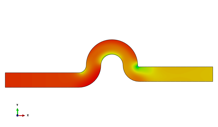
In the toolbox, click ![]() to open the Contour Plot Options dialog box. Toggle on Continuous under Contour Intervals, and click Apply.
to open the Contour Plot Options dialog box. Toggle on Continuous under Contour Intervals, and click Apply.
Abaqus/CAE creates a smooth pressure contour plot, as shown in Figure E–15.
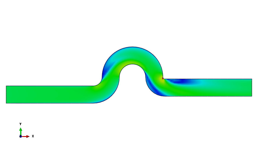
Using the Field Output toolbar, select V as the output variable to plot.
A contour plot of the velocity magnitude appears, as shown in Figure E–16.
In the toolbox, click ![]() to create a time history animation. Select an output variable (velocity, pressure, etc.) to animate the results.
to create a time history animation. Select an output variable (velocity, pressure, etc.) to animate the results.
Plot the turbulence variables.
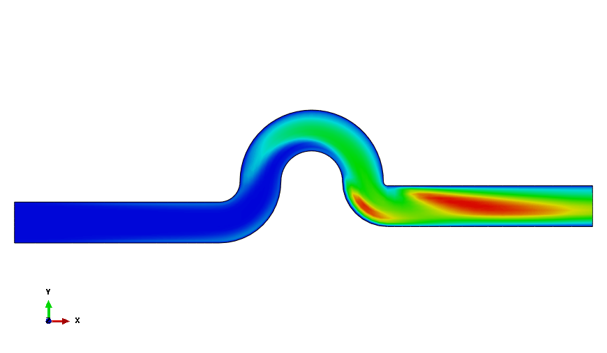
Using the Field Output toolbar, select TURBNU as the output variable.
Abaqus/CAE displays a smooth contour plot of turbulent viscosity, as shown in Figure E–17.
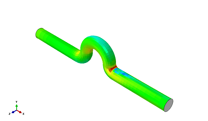
Toggle off the view cut by clicking the View cut tool ![]() .
.
From the Views toolbar, select the isometric view.
Using the Field Output toolbar, select YPLUS as the output variable.
Abaqus/CAE creates a smooth contour plot of nondimensional wall distance on the wall surface, as shown in Figure E–18.
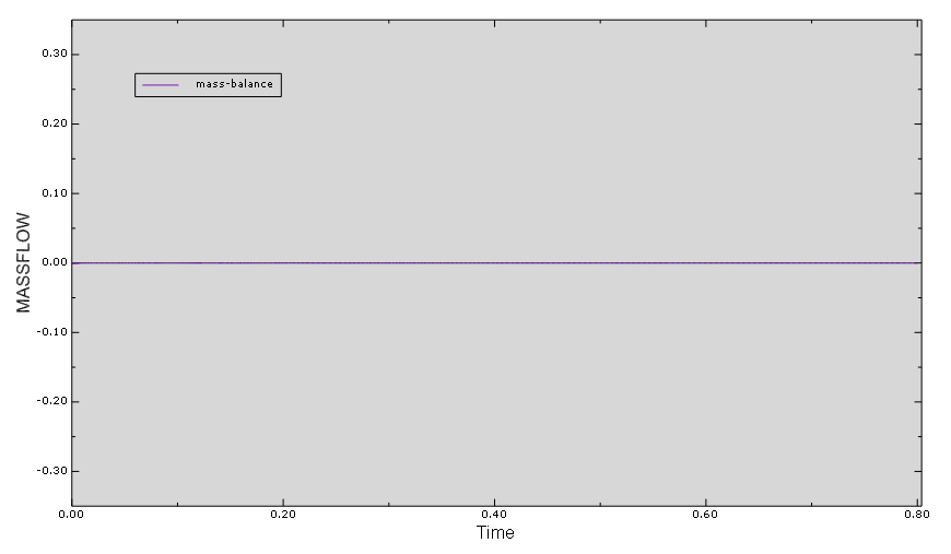
Verify the mass balance.
Select Tools![]() XY Data
XY Data![]() Create.
Create.
In the Create XY Data dialog box that appears, select ODB history output as the source, and click Continue.
In the History Output dialog box, select the MASSFLOW output at the inlet and outlet and click Plot, as shown in Figure E–19.
In the History Output dialog box, click Save As.
In the Save XY Data As dialog box, select sum as the Save Operation, name the new X–Y data object mass-balance, and click OK.
Abaqus/CAE creates a plot representing the sum of mass flow rates at the inlet and the outlet surfaces, as shown in Figure E–20. The plot verifies that inlet and outlet mass flow rates are balanced.