Product: Abaqus/Standard
This example shows how you can investigate the flexibility of a substructure in your model during a dynamic analysis.
The following abaqus adams translator features are demonstrated:
creating Abaqus models of MSC.ADAMS components,
converting the Abaqus results into an MSC.ADAMS modal neutral (.mnf) file, the format required by ADAMS/Flex, and
displaying results of an ADAMS/Flex flexibility analysis.
The following cases are illustrated:
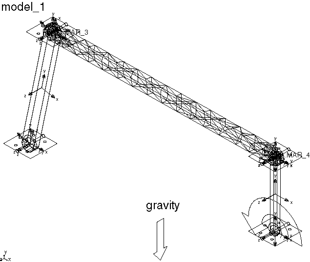
A three-dimensional steel link substructure meshed with solid elements and with displacement degrees of freedom at its nodes, as shown in Figure 15.1.7–1. Multi-point constraints connect it to the other components in the model. The analysis includes two steps: an eigenfrequency extraction step and a substructure generation step defined for a flexible body.
The same steel link meshed with beam elements. Because the beam elements have both displacement and rotational degrees of freedom at their nodes, no multi-point constraints are required to connect the substructure to the rest of the model. The analysis includes two steps: an eigenfrequency extraction step and a substructure generation step defined for a flexible body.
Both cases described in this section share the same general approach:
Create an Abaqus model for each flexible component of the MSC.ADAMS model. Each component is modeled as an Abaqus substructure.
Run the Abaqus analysis.
Run the abaqus adams translator to read the Abaqus results from the SIM database produced by the analysis and to create the modal neutral (.mnf) file for MSC.ADAMS.
Read the modal neutral file into MSC.ADAMS. A separate modal neutral file must be created for each flexible part in MSC.ADAMS.
This example models a simple flexible link component using three-dimensional continuum elements.
The example includes an eigenfrequency extraction and a substructure generation analysis.
The steel used in this case has a Young's modulus of 2.07 × 10¹¹ N/m2 (3.0 × 10⁷ lbf/in2) and a Poisson’s ratio of 0.29. The density of the model is 7.8 × 10³.
This analysis includes two multi-point constraints: one applied to the LEFTCYL node set and the other applied to the RIGHTCYL node set.
The analysis includes two steps: an eigenfrequency extraction step and a substructure generation analysis step.
Element stiffness matrices and mass matrices are written to the SIM database for the element set PROP1 as part of the substructure generation analysis step.
You can perform the analysis of the link with solid elements using the procedure shown below.
Enter the following commands to extract the input files from the compressed archive files provided with the Abaqus release:
abaqus fetch job=adams_ex1
abaqus fetch job=adams_ex1_nodes
abaqus fetch job=adams_ex1_elements
Enter the following command to execute the Abaqus analysis:
abaqus job=adams_ex1
Enter the following command to execute the abaqus adams translator and translate the results in a SIM database generated in the Abaqus analysis to a modal neutral file for use with ADAMS/Flex:
abaqus adams job=adams_ex1 substructure_sim=adams_ex1_Z1
Because the solid elements have only displacement degrees of freedom at their nodes, multi-point constraints are used to provide a connection to the other components in the MSC.ADAMS model. Two nodes are added along the centerline of the beam at the centers of the hinge holes. The C3D10 nodes that lie on the faces of the hinge holes are connected to the extra nodes with BEAM-type multi-point constraints, allowing the nodes to transmit both forces and moments between the link and other MSC.ADAMS components.
The options used to define the single substructure are those described in “The Abaqus substructure model” in “Translating Abaqus data to MSC.ADAMS modal neutral files,” Section 3.2.38 of the Abaqus Analysis User's Guide. Twenty fixed-interface vibration modes are computed to represent the dynamic behavior of the link.
MSC.ADAMS uses the fixed-interface vibration modes and the constraint modes to characterize the flexibility of the link. The eight lowest fixed-interface vibration frequencies computed by Abaqus are shown in Table 15.1.7–1. These frequencies are reported in the adams_ex1.dat file. The abaqus adams translator combines these fixed-interface modes with the static constraint modes to compute an equivalent modal basis to be used by ADAMS/Flex. The first six frequencies of this equivalent basis are approximately zero. The next eight frequencies for the unconstrained model are shown in Table 15.1.7–2. These frequencies are written to the screen when executing the abaqus adams translator.
This example models a simple flexible link component using three-dimensional beam elements.
As in Case 1, this example includes an eigenfrequency extraction and a substructure generation analysis.
The beam elements have both displacement and rotational degrees of freedom at their nodes.
The analysis includes two steps: an eigenfrequency extraction step and a substructure generation analysis step.
You can perform the analysis of the link with beam elements using the procedure shown below.
Enter the following command to extract the input files from the compressed archive files provided with the Abaqus release:
abaqus fetch job=adams_ex2
Enter the following command to execute the Abaqus analysis:
abaqus job=adams_ex2
Enter the following command to execute the abaqus adams translator and translate the results in a SIM database generated in the Abaqus analysis to a modal neutral file for use with ADAMS/Flex:
abaqus adams job=adams_ex2 substructure_sim=adams_ex2_Z1
The primary difference between the beam model and the solid model is that the beam model uses only 10 B31 elements (11 nodes). Because the beam elements have both displacement and rotational degrees of freedom at their nodes, no multi-point constraints are needed to connect the link to other MSC.ADAMS components. The rest of the model is essentially identical to the solid model of the link.
The first eight nonzero frequencies for the unconstrained model are shown in Table 15.1.7–3. These frequencies are close to those of the solid model of the link. Although the computational cost in Abaqus is much less for this model than for the solid model, the computational costs in MSC.ADAMS for the two models are very similar because both models have 32 modes (12 constraint modes and 20 fixed-interface vibration modes).
Input file to analyze a link model subjected to a gravity load.
Node definitions for Case 1.
Element definitions for Case 1.
Input file to analyze a link model subjected to a gravity load.