Products: Abaqus/Standard Abaqus/CAE
This example uses the Optimization module to optimize the stiffness of a simple plate by introducing stiffening beads.
This example illustrates condition-based bead optimization of a simply supported plate. During a bead optimization, the nodes of the shell elements are moved in the direction of the shell normal to increase the moment of inertia, which leads to a greater stiffness or higher eigenfrequencies. The resulting beads are easy to reproduce in a sheet metal stamping process without increasing the mass or cost of the finished product. For more information, see “Bead optimization” in “Structural optimization: overview,” Section 13.1.1 of the Abaqus Analysis User's Guide.
The plate is a 600 mm × 600 mm three-dimensional shell part. A shell section is assigned to the part with a thickness of 1.5 mm. The shell section uses the default Simpson integral rule with five integration points through the shell section.
The plate is made of an elastic material with a Young's modulus of 210 GPa and a Poisson’s ratio of 0.3.
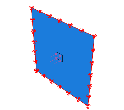
The edges of the plate are fixed in all three translation degrees of freedom. A pressure of 1.0 is applied to a partitioned region at the center of the plate, as shown in Figure 11.4.1–1.
The bead optimization is configured as described in the following sections.
This example creates a bead optimization task that is governed by the condition-based optimization algorithm. The bead width is specified as 60 mm.
The entire plate is selected as the design area. By default, the Optimization module freezes the position of the nodes around the edge of the plate that were included in the boundary condition.
A design response is created that calculates the maximum of the strain energy over all the elements in the design area. A second design response calculates the bead height.
A single objective function attempts to minimize the maximum of the strain energy of the design area. Since compliance is defined as the sum of the strain energy, and stiffness is the reciprocal of compliance, the objective function is equivalent to maximizing the stiffness of the plate.
The example creates an optimization process with the default maximum of three design cycles.
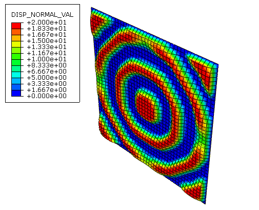
A Python script is included that reproduces the model using the Abaqus Scripting Interface in Abaqus/CAE. The Python script (plate_bead_optimization.py) builds the optimization model and executes the optimization job. To view the results of the optimization, you can use the Optimization Process Manager to combine the output database files that are generated and open the resulting output database file (Beadprocess\TOSCA_POST\BeadJob_post.odb). You can use the Visualization module to display a contour plot of the optimized nodal displacement (DISP_NORMAL_VAL) that shows the generated stiffening beads. You can return to the Optimization module to review the bead optimization model that was created in Abaqus/CAE.
The Python script can be run interactively or from the command line, and the script must be available from your working directory.
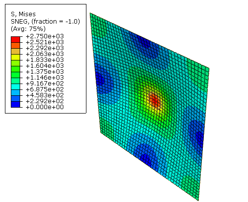
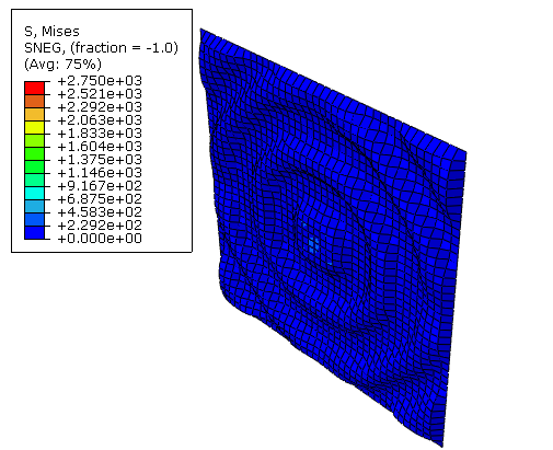
The results are available in the combined output database file created from the Optimization Process Manager. The step contains three optimization iterations that correspond to the three design cycles of the optimization process. Figure 11.4.1–2 shows how the bead optimization moves nodes to create stiffening beads along the bending trajectories. Figure 11.4.1–3 and Figure 11.4.1–4 compare the plate stresses prior to the optimization and after the introduction of the stiffening beads.