Products: Abaqus/Standard Abaqus/CAE
This example uses the Optimization module to minimize the stress concentrations in a connecting rod without changing the volume of the connecting rod.
This example illustrates shape optimization of a connecting rod. Shape optimization makes slight modifications to the position of the surface nodes in the design area to achieve the optimized solution. Shape optimization is typically applied at the end of the design process when the general outline of a component is fixed and only minor changes are allowed. For more information, see “Shape optimization” in “Structural optimization: overview,” Section 13.1.1 of the Abaqus Analysis User's Guide.
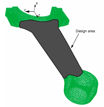
The connecting rod model is a single orphan mesh part that was meshed with linear tetrahedral (C3D4) elements. The connecting rod is symmetric about the X–Z plane.
The connecting rod is made of an elastic material with a Young's modulus of 210 GPa, a Poisson’s ratio of 0.3, and a density of 7800 kg/m3.
The displacement of the center node of the small end is constrained in the x- and y-directions, and the rotation of the center node is constrained in the y- and z-directions. For the center node of the big end, the displacement in the x- and z-directions and the rotation in the y- and z-directions are constrained.
During the first step a 25000 N load is applied to the center node of the small end of the connecting rod in the z-direction.
During the second step a 2000 N load is applied to the center node of the small end of the connecting rod in the z-direction and a 1750 N load is applied to the center node of the big end of the connecting rod in the y-direction. In addition, a rotation of 0.004 radians about the x-axis is applied to the center node of the big end.
The shape optimization is configured as described in the following sections.
This example creates a shape optimization task. To ensure good quality elements in the final design, mesh smoothing is applied to the elements in the design area.
The design area of the model is the region that will be modified during the optimization, as shown in Figure 11.2.1–1. Regions are excluded from the design area because they are required for fixtures and for applying loads.
A design response is created for each step that determines the maximum von Mises stress in the design area. A third design response calculates the volume of the design area.
The objective function determines which of the two design responses results in the largest von Mises stress in the design nodes. The objective function then tries to minimize the maximum von Mises stress for that design response.
The volume design response is configured as the single optimization constraint such that the total volume of the design area remains unchanged during the optimization process.
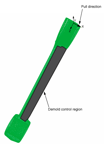
The example introduces a casting restriction by defining demold control geometry restrictions that are applied to the nodes in each half of the design area in the positive x- and negative x-directions. Figure 11.2.1–2 illustrates the demold control geometry restriction that is applied to one half of the design area in the positive x-direction.
This example imports the model in the form of an orphan mesh from an input file. The input file contains the element sets that are used to define the regions of the model that are used by the optimization, such as the design area and the demold control region. The example creates an optimization process with a global stop criterion of 15 design cycles. To maintain the quality of the surface elements, mesh smoothing is applied to the design area, which adjusts the position of the inner nodes in relation to the movement of the surface nodes. For more information, see “Applying mesh smoothing to a shape optimization” in “Structural optimization: overview,” Section 13.1.1 of the Abaqus Analysis User's Guide.
The center nodes at both the ends of the connecting rod are connected to the bearing surfaces of the connecting rod with kinematic couplings.
A Python script is included that reproduces the model using the Abaqus Scripting Interface in Abaqus/CAE. The Python script (conrod_shape_optimization.py) imports the input file (connecting_rod.inp) and builds the optimization model. The script can be run interactively or from the command line. Both the Python script and the input file must be available from your working directory.
When the script completes, you can use the Optimization module to review the shape optimization model that was created in Abaqus/CAE. To run the optimization, you can submit the optimization process from the Optimization Process Manager in the Job module. You can use the Optimization Process Manager to monitor the progression of the optimization and to view the results of the shape optimization in the Visualization module.
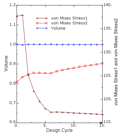
The results are available in the output database file created by the optimization process. The step contains 15 optimization iterations that correspond with the 15 design cycles of the optimization process. Figure 11.2.1–3 shows a history output plot of the von Mises stress design response for each of the two load cases over the 15 design cycles. The history output plot also shows the volume design response, which is kept constant throughout the optimization.
The position of the surface nodes in the design area is optimized such that for the specified volume constraint and geometry restrictions the von Mises stress is minimized during the load case that results in the maximum stress. In this example the 25000 N load that is applied to the small end in the first step results in the highest von Mises stress in the connecting rod. Therefore, the objective function adjusts the surface nodes to reduce the maximum von Mises stress during the first step, although the resulting optimized shape allows the von Mises stress to increase slightly under the loading conditions in the second step.
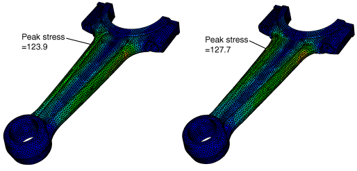
Figure 11.2.1–4 shows the initial von Mises stress distribution during the first load case and the change in the stress distribution after 15 design cycles. Figure 11.2.1–5 shows similar von Mises stress distribution plots before and after optimization during the second load case.
Script to create the model and the optimization attributes using connecting_rod.inp.
Input file to create the orphan mesh connecting rod and the element sets that are used by the optimization.