Product: Abaqus/Standard
This example illustrates how you can effectively couple Moldflow and Abaqus.
The following features of the abaqus moldflow translator are demonstrated:
transforming finite element model information from a Moldflow analysis into a partial Abaqus input file,
adding appropriate data for the analysis,
performing natural frequency analyses, and
calculating deformation due to initial stresses.
The results of a Moldflow simulation, which models the plastics injection mold-filling process, include calculations of material properties and residual stresses in the plastic part. Two types of parts, a filled bracket and an unfilled bracket, are studied in this example to illustrate how you can transform finite element model information from a Moldflow simulation into a partial Abaqus input file, adding boundary conditions and step data, and requesting output.
This example illustrates the use of the abaqus moldflow translator.
The three cases share the same general approach. The following procedure summarizes the typical usage of the abaqus moldflow translator:
Export the data from Moldflow simulation as follows:
For a midplane Moldflow simulation, export the finite element mesh data to a file named job-name.pat and the results data (material properties and residual stresses) to a file named job-name.osp.
For a three-dimensional solid Moldflow simulation using Moldflow Version MPI 6, run the Visual Basic script mpi2abq.vbs to export the finite element mesh data to a file named job-name_mesh.inp and the results data to .xml files.
Run the abaqus moldflow translator to create a partial Abaqus input (.inp) file from the Moldflow interface files.
Edit the Abaqus input file to add appropriate data for the analysis (for example, add boundary conditions and step data).
Submit the Abaqus input file for analysis.
All files associated with these analyses are included with the Abaqus release; you can use the Abaqus fetch utility to extract example problem files from the compressed archive files.
To extract all the relevant files for a particular example problem, enter the following commands:
| Case 1 | abaqus fetch job=moldflow_ex1* |
| Case 2 | abaqus fetch job=moldflow_ex2* |
| Case 3 | abaqus fetch job=bracket3d_mpi6* |
For information on using wildcard expressions with the Abaqus fetch utility, see “Fetching sample input files,” Section 3.2.17 of the Abaqus Analysis User's Guide.
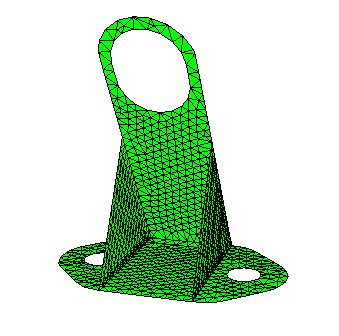
The bracket in Case 1 consists of 926 nodes and 1719 S3R elements. The model contains seven different element sets. Each element set has a different thickness and is modeled as a laminated composite with 20 layers.
Ten unrestrained vibration modes are computed. The first six frequencies are approximately zero. The frequencies for the first four flexible modes are listed in Table 1.3.19–1.
The Abaqus finite element model is shown in Figure 1.3.19–1.
Case 2 uses the same Abaqus finite element model as Case 1, but the material properties are transversely isotropic. The shell section definition is homogeneous instead of composite. Twenty-one equally spaced Simpson integration points are used through the shell thickness.
The frequencies for the first four flexible vibration modes of the unfilled bracket are listed in Table 1.3.19–2. The unfilled material in this example is softer than the filled material in Case 1; consequently, the frequencies are lower.
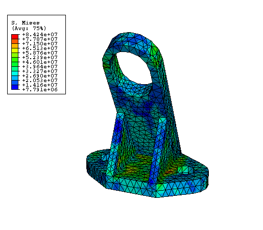
Case 3 uses a solid Abaqus finite element model that is similar to the model used in Case 1.
To execute the abaqus moldflow translator, enter the following command:
abaqus moldflow job=bracket3d_mpi6 3D initial_stress=on
A contour plot of initial stresses is shown in Figure 1.3.19–2.
Input file to analyze a fiber-filled bracket.
Input file to analyze an unfilled bracket.